Estimation of Noisy Logistic Dynamical Map by Using
Neural Network with FFT Transfer Function
Salah H. Abid
*, Saad S. Mahmood, Yaseen A. Oraibi
Department of Mathematics, College of Education, AL-Mustansiriyah University, Baghdad, Iraq
Abstract
The aim of this paper is to design a feed forward artificial neural network (Ann) to estimate one dimensional
noisy Logistic dynamical map by selecting an appropriate network, transfer function and node weights to get noisy Logistic
dynamical map estimation. The proposed network side by side with using Fast Fourier Transform (FFT) as transfer function
is used. For different cases of the system, noisy deterministic, noisy chaotic and noise high chaotic, the experimental results
of proposed algorithm will compared empirically, by means of the mean square error (MSE) with the results of the same
network but with traditional transfer functions, Logsig and Tagsig. The performance of proposed algorithm is best from
others in all cases from Both sides, speed and accuracy.
Keywords
FFT, Logsig, Tagsig, Feed Forward neural network, Transfer function, Noisy Logistic map, Uniform noise,
Noise normal, Logistic noise
1. Introduction
Ann is a simplified mathematical model of the human
brain, It can be implemented by both electric elements and
computer software. It is a parallel distributed processor with
large numbers of connections, it is an information processing
system that has certain performance characters in common
with biological neural networks. Ann has been developed as
generalizations of mathematical models of human cognition
or neural biology, based on the assumptions that:
1- Information processing occurs at many simple
elements called neurons that are fundamental to the
operation of Ann's.
2- Signals are passed between neurons over connection
links.
3- Each connection link has an associated weight which,
in a typical neural net, multiplies the signal
transmitted.
4- Each neuron applies an action function (usually
nonlinear) to its net input (sum of weighted input
signals) to determine its output signal [15].
The units in a network are organized into a given topology
by a set of connections, or weights.
Ann is characterized by [30]:
* Corresponding author:
[email protected] (Salah H. Abid) Published online at http://journal.sapub.org/ajcam
Copyright©2019The Author(s).PublishedbyScientific&AcademicPublishing This work is licensed under the Creative Commons Attribution International License (CC BY). http://creativecommons.org/licenses/by/4.0/
1- Architecture: its pattern of connections between the
neurons.
2- Training Algorithm: its method of determining the
weights on the connections.
3- Activation function.
Ann are often classified as single layer or multilayer. In
determining the number of layers, the input units are not
counted as a layer, because they perform no computation.
Equivalently, the number of layers in the net can be defined
to be the number of layers of weighted interconnects links
between the slabs of neurons [46].
1.1. Multilayer Feed Forward Architecture [22]
In a layered neural network the neurons are organized in
the form of layers. We have at least two layers: an input and
an output layer. The layers between the input and the output
layer (if any) are called hidden layers, whose computation
nodes are correspondingly called hidden neurons or hidden
units. Extra hidden neurons raise the network’s ability to
extract higher-order statistics from (input) data.
The Ann is said to be fully
connected
in the sense that
every node in each layer of the network is connected to every
other node in the adjacent forward layer; otherwise the
network is called partially connected. Each layer consists of
a certain number of neurons; each neuron is connected to
other neurons of the previous layer through adaptable
synaptic weights w and biases b.
1.2. Literature Review
non-linear dynamical systems from data. Emphasis is placed
on predictions at long times, with limited data availability.
Inspired by global stability analysis, and the observation of
strong correlation between the local error and the maximal
singular value of the Jacobian of the ANN, they introduced
Jacobian regularization in the loss function. This
regularization suppresses the sensitivity of the prediction to
the local error and is shown to improve accuracy and
robustness. Comparison between the proposed approach and
sparse polynomial regression is presented in numerical
examples ranging from simple ODE systems to nonlinear
PDE systems including vortex shedding behind a cylinder,
and instability-driven buoyant mixing ow. Furthermore,
limitations of feedforward neural networks are highlighted,
especially when the training data does not include a low
dimensional attractor. The need to model dynamical
behavior from data is pervasive across science and
engineering. Applications are found in diverse fields such as
in control systems [43], time series modeling [41], and
describing the evolution of coherent structures [12]. While
data-driven modeling of dynamical systems can be broadly
classified as a special case of system identification [23], it
is important to note certain distinguishing qualities: the
learning process may be performed off-line, physical
systems may involve very high dimensions, and the goal may
involve the prediction of long-time behavior from limited
training data. Artificial neural networks (ANN) have
attracted considerable attention in recent years in domains
such as image recognition in computer vision [17, 37] and in
control applications [12]. The success of ANNs arises
from their ability to effectively learn low-dimensional
representations from complex data and in building
relationships between features and outputs. Neural networks
with a single hidden layer and nonlinear activation function
are guaranteed to be able to predict any Borel measurable
function to any degree of accuracy on a compact domain [16].
The idea of leveraging neural networks to model dynamical
systems has been explored since the 1990s. ANNs are
prevalent in the system identification and time series
modeling community [19, 28, 29, 35], where the mapping
between inputs and outputs is of prime interest. Billings et al.
[5] explored connections between neural networks and the
nonlinear autoregressive moving average model (NARMAX)
with exogenous inputs. It was shown that neural networks
with one hidden layer and sigmoid activation function
represent an infinite series consisting of polynomials of the
input and state units. Elanayar and Shin [13] proposed the
approximation of nonlinear stochastic dynamical systems
using radial basis feedforward neural networks. Early work
using neural networks to forecast multivariate time series of
commodity prices [9] demonstrated its ability to model
stochastic systems without knowledge of the underlying
governing equations. Tsung and Cottrell [44] proposed
learning the dynamics in phase space using a feedforward
neural network with time-delayed coordinates. Paez and
1.3. Fast Fourier Transform
The first to propose the techniques that we now call the
fast Fourier transform (FFT) for calculating the coefficients
in a trigonometric expansion of an asteroid’s orbit in 1805
[8]. However, Fast Fourier transform is an algorithm that
calculates the value of the discret Fourier transform in faster.
the speed this algorithm Is due to the fact that it does not
calculate the parts that are equal to zero. the algorithm is
discovered by James W. Cooley and John W. Tukey who
published the algorithm in 1965 [11]
As know today
𝑥 𝑡 =
21𝑎
0+
∞𝑛=1(𝑎
𝑛𝑐𝑜𝑠
𝜋𝑛𝐿𝑡
+ 𝑏
𝑛𝑠𝑖𝑛
𝜋𝑛𝐿𝑡) (1)
The coefficients can be datermain as follows :
𝑎𝑛
=
1𝐿𝑥 𝑡 𝑐𝑜𝑠
−𝐿𝐿 𝜋𝑛𝐿𝑡 𝑑𝑡
(2)
𝑏𝑛
=
1𝐿𝑥 𝑡 𝑠𝑖𝑛
−𝐿𝐿 𝜋𝑛𝐿𝑡 𝑑𝑡
(3)
𝑎
0=
1𝐿𝑥 𝑡 𝑑𝑡
−𝐿𝐿(4)
The discrete Fourier transform (DFT) is one of the most
powerful tools in Digital signal processing. The DFT
enables us to conveniently analyze and Design systems in
frequency domain [1] and the formal as:
𝑋𝑘
=
𝑁−1𝑛=1𝑥𝑛
𝑒
−𝑗2𝜋𝑁𝑛𝑘(5)
2. Logistic Map
In 1845, Pierre Verhulst proposed a logistic map, which is
a simple non-linear dynamical map. A logistic map is one of
the most popular and simplest chaotic maps. Logistic map
became very popular after it was exploited in 1979 by the
biologist Robert M. May [24] [21]. The logistic map is a
polynomial mapping, a complex chaotic system, the
behaviour of which can arise from very simple non-linear
dynamical equations. The logistic map equation is written as
[26]:
𝐺(𝑥) = 𝑥𝑛+1
= 𝑟𝑥𝑛
1 − 𝑥
𝑛(6)
𝑥
1= 𝑟𝑥
01 − 𝑥
0𝑥2
= 𝑟𝑥1
1 − 𝑥
1…
𝑥
2= 𝑟
2𝑥
01 − 𝑥
01 − 𝑟𝑥
0+ 𝑟𝑥
02where x
nis a number between zero and one, x
0represents the
initial population, and r is a positive number between zero
and four.
The logistic map is one of the chaotic maps; it is highly
sensitive to change in its parameter value, where a different
value of the parameter r will produce a different sketches. Its
transformation function is
𝑓: 0,1 → 0,1 which is defined
in the above equation (6). From the onset of chaos, a
seemingly random jumble of dots, the behavior of the
logistic map depends mainly on the values of two variables
(r, x
0); by changing one or both variables’ values we can
observe different logistic map behavior’s. The population of
a logistic map will die out if the value of r is between 0 and 1,
and the population will be quickly stabilized on the value (1-
r )/r if the value of r is between 1 and 3. Then, the population
will oscillate between two values if the value of parameter
r is between 3 and 3.45. After that, with values of parameter
r between 3.45 and 4 the periodic fluctuation becomes
significantly more complicated. Finally, most of the values
after 3.57 show chaotic behaviour.
In the logistic map
𝑔(𝑥𝑛
) = 𝑟𝑥𝑛
1 − 𝑥
𝑛, the function
result depends on the value of parameter r, where different
values of r will give quite different pictures. We can note that
g(x
1) = x
2and g(x
2) = x
1, that mean g(g(x
2)) = x
1and g(g(x
1))
= x
2. According to Alligood et al. (1996) the periodic
fluctuation between x
1, x
2is steady and attracts orbits
(trajectories). Therefore, there are a minimum number of
iterations of the
orbit to repeat the point. There are
obvious
differences between the behaviour of the exponential model
and the logistic model’s behaviour. [24, 21]
Figure 1. Bifurcation diagram of the Logistic map [26]
2.1. Noisy Logistic map (NG) Solution
In this section we will explain how this approach can be
used to find the approximate solution of the noisy logistic
map that is stated in equation (6).
NG(x) is the solution to be computed. Let y
t(x, p) denotes
a trial solution with adjustable parameters p.
In the proposed approach, the trial solution y
temploys a
FFNN and the parameters p corresponding to the weights
and biases of the neural architecture. We choose a form for
the trial function y
t(x) such that y
t(x,p) = N(x, p) where N(x,
p) is a single-output FFNN with parameters (weights) p and n
input units fed with the input vector x.
2.2. Computation of the Gradient
The error corresponding to each input vector x
iis the value
E (x
i) which has to force near zero. Computation of this error
value involves not only the FFNN output but also the
derivatives of the output with respect to any of its inputs.
Therefore, for computation the gradient of the error with
respect to the network weights, consider a multilayer FFNN
with n input units (where n is the dimensions of the domain),
two hidden layer with H sigmoid units,q hidden layer and a
linear output unit.
For a given input vector x
( x
1, x
2, …, x
n) the output of
N
𝐻𝑖=1𝑣𝑘
𝜎(𝑢𝑖)
, z
i
n
ij j i j 1
w x
b
and
𝑢𝑘=
𝑞𝑘=1𝑠𝑖𝑘
𝜎 𝑧𝑗 + 𝑏𝑖𝑘
w
ijdenotes the weight connecting the input unit j to the
hidden unit i
𝑠𝑖𝑘
denotes the weight connecting the hidden unit i to the
hidden unit k
v
kdenotes the weight connecting the hidden unit k to the
out put unit,
b
idenotes the bias of hidden unit i,
b
ikdenotes the bias of hidden unit i to the hidden unit k,
and
σ is the transfer function
The gradient of suggest FFNN, with respect to the
coefficients of the FFNN can be computed as:
𝜕𝑁
𝜕𝑣𝑘
= 𝜎(𝑢𝑖), (7)
𝜕𝑁
𝜕𝑏𝑖
= 𝑣𝑘𝜎′(𝑢𝑖), (8)
𝜕𝑁𝜕𝑤𝑖𝑗
= 𝑣
𝑘𝜎′(𝑢
𝑖)𝑥
𝑗, (9)
𝜕𝑁𝜕𝑠𝑖𝑘
= 𝑣𝑘
𝜎(𝑧
𝑗)𝜎′(𝑢𝑖)𝑥𝑗
, (10)
𝜕𝑁𝜕𝑏𝑖𝑘
= 𝑣
𝑘𝑠
𝑖𝑘𝜎′(𝑢
𝑖)𝜎′(𝑧
𝑗), (11)
The derivative of the error performance with respect to
the FFNN coefficients can be defined and then it is easy to
find minimization solution.
3. Suggested Networks
It is well known that a multilayer FFNN consist one
hidden layer can approximate any function to any accuracy
[27], but dynamical maps they have more completed
behavior than other functions, thus, we suggest FFNN
contains two hidden layer, one input and one output to
estimate a solution for dynamic maps.
The suggested network divided the inputs in to two parts
60% for training and 40% for testing. The error quantity to be
minimized is given by:
E[p]
n
i
1
{NG(xi) – y
t(x
i) }
2, (12)
Where x
i
[0, 1]. It is easy to evaluate the gradient of the
performance with respect to the coefficient. Using (7) – (11).
The training progress algorithm of FFNN with supervises
training and BFGS algorithm is given as follows. Assume
that there are one nodes in the First layer (input layer), the
second layer (hidden layer) consist with ten nodes, the third
layer (hidden layer) consist with five
nodes and the fourth
layer (output layer) consist with one node.
Following the steps of the technique as an algorithm,
Step 0:
input and target.
Insert the input (x: x
1, x
2, x
3,…., x
n) and the target.
Step 1:
allocating inputs.
Each input goes to each neurons with a hidden layer.
Step 2:
initialization weights.
We initial weights and bias from the uniform distribution
respectively for all connection in the neural network.
Step 3:
select the following.
- parameter epoch
- parameter goal (𝜀)
- performance function (MSE)
Step 4:
calculations in each node in the first hidden layer.
In each node in hidden layer, computing the sum of the
product of weights and inputs and adding the result to the
bias.
Step 5:
compute the output of each node for the first
hidden layer.
Take the active function for sum value in step4, then its
output is sent to the second hidden layer as input.
Step 6
: calculations in each node in the second layer.
In each node in second hidden layer, computing the sum
of the product of weights and inputs and adding the result to
the bias.
Step 7:
compute the output of each node for the second
hidden layer.
Take the active function for sum value in step 6, then its
output is sent to the output layer as input.
Step 8:
calculations in output layer.
There is only one neuron (node) in the output layer. The
node sum is the product of weights by inputs.
Step 9:
compute the output of node in output layer
The value of active function for node output is also
considered as the output of overall network.
Step 10:
compute the mean square error (MSE).
The mean square error is computed as follows
MSE =
𝑛1 𝑛𝑟=0𝑒𝑟
2where
𝑒𝑟
= 𝑡𝑟
− 𝑦
𝑟the MSE is a measure of performance.
Step 11:
The checking.
When
𝑀𝑆𝐸 ≤ 𝜀 such that
𝜀 is small value close to zero,
then stop the training and the bias and weights are sent.
Otherwise training process goes to the next step.
Step 12:
when select the training rule, the low for update
weights and bias between the hidden layer and the output
layer are calculated
Step 13:
the update weights and bias in output layer.
At end for each iteration, the weights and bias are
updating as follows:
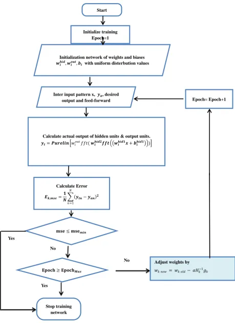
Figure 2. Flowchart for training algorithm with BFGS
Start
Initialize training
Epoch=1
Inter input pattern x,
𝒚
𝒂, desired
output and feed-forward
Initialization network of weights and biases
𝒘
𝒊𝒉𝒊𝒅, 𝒘
𝒊𝒐𝒖𝒕, 𝒃
𝒊with uniform disterbution values
𝒚
𝒕= 𝑷𝒖𝒓𝒆𝒍𝒊𝒏 𝑤
𝑖𝑜𝑢𝑡𝑓𝑓𝑡( 𝒘
𝒊𝒉𝒊𝒅𝟐𝒇𝒇𝒕 𝒘
𝒊𝒉𝒊𝒅𝟏𝒙 + 𝒃
𝒊𝒉𝒊𝒅𝟏)
Calculate actual output of hidden units & output units.
𝑬
𝒌,𝒎𝒔𝒆=
𝟏
𝑵
𝒚
𝒕𝒏− 𝒚
𝒂𝒏 𝟐𝑁
𝑛=1
Calculate Error
𝐦𝐬𝐞 ≤ 𝐦𝐬𝐞
𝒎𝒊𝒏𝐄𝐩𝐨𝐜𝐡 ≥ 𝐄𝐩𝐨𝐜𝐡
𝑴𝒂𝒙Stop training
network
Yes
No
Yes
No
𝑤
𝑘 𝑛𝑒𝑤= 𝑤
𝑘 𝑜𝑙𝑑− 𝛼𝐻
𝑘−1𝑔
𝑘Adjust weights by
When (new) means the current iteration and (old) means
the previous iteration,
𝑔𝑘 represent the gradient for weights and bias,
𝛼 is the
parameter selected to minimize the performance function
along the search direction,
𝐻
𝑘−1represent the invers
hessian matrix, v is the weight in the output layer and b is
the bias.
Step 14: the update of weights and bias in the first hidden
layer.
Each hidden node in the first hidden layer updates the
weights and bias as follow:
𝑤𝑘 𝑛𝑒𝑤
= 𝑤𝑘 𝑜𝑙𝑑
− 𝛼𝐻
𝑘−1𝑔𝑘
𝑏𝑘 𝑛𝑒𝑤
= 𝑏𝑘 𝑜𝑙𝑑
− 𝛼𝐻𝑘
−1𝑔𝑘
Where w is the weight of hidden layer and b is the bias.
Step 15: the update of weights and bias in the second
hidden layer as follow.
𝑠𝑘 𝑛𝑒𝑤
= 𝑠𝑘 𝑜𝑙𝑑
− 𝛼𝐻
𝑘−1𝑔𝑘
𝑏𝑘 𝑛𝑒𝑤
= 𝑏𝑘 𝑜𝑙𝑑
− 𝛼𝐻𝑘
−1𝑔𝑘
Where s is the weight of hidden layer and b is the bias.
Step 16:
return to step2 for next iteration.
4. Data Description
We know that for each starting point in dynamical map
there are a minimum number of iterations of the orbit to
repeat a point. So we choose number of initial points and
iterated until reaching a point. There are initial points have
thousands of iterations until reaching a point a gain, but the
ability of personal computer will restrict us to take all these
points. In addition, the higher value of the Bifurcation
parameter implicit to complicate the calculations. For that
reason, we will take the maximum capacity of the computer
which is a one hundred point for initial point exceeding 100
iterations distributed on all the domain map evenly and the
number of iterations of points was found by the program
MATLAB R2010a.
4.1. Training for Noisy Logistic Map
To design FFNN that is not sensitive to noise for this case,
we use the propose network with FFT as transfer function to
train the data with noise, it is suitable to choose the
maximum number of epochs, when the noisy data have noise
of (uniform, normal and logistic) distributions and we take
for all noises value of variance (0.05, 0.5, 15). We train this
case with noise with three types of transfer functions Tansig,
logsig and FFT. It is worth to mention that the run size is
k=1000.
4.2. Uniform Distribution [36]
A uniform distribution is one have a constant probability.
The probability density function and cumulative distribution
function for continuous uniform distribution on the interval
[a, b] are
𝑃 𝑥 =
𝑏−𝑎1𝑓𝑜𝑟 𝑎 ≤ 𝑥 ≤ 𝑏
0 𝑜. 𝑤
(13)
𝐷 𝑥 =
0 𝑓𝑜𝑟 𝑥 < 𝑎
𝑥−𝑎𝑏−𝑎
𝑓𝑜𝑟 𝑎 ≤ 𝑥 ≤ 𝑏
1 𝑓𝑜𝑟 𝑥 > 𝑏
(14)
One can generate values from Uniform random variable as
follows,
U = rand (1:q) * 12𝑣 (15)
Where q is represent the number point and v is represent
the variance.
4.3. Normal Distribution [36]
Let x be a normally distributed random variable with mean
−∞ < 𝜇 < ∞ and variance
0 < 𝜎
2, where
𝑥 ∈ (−∞, ∞)
with probability density function and cumulative distribution
function are respectively,
𝑃 𝑥 =
𝜎 2𝜋1∗ 𝑒
−(𝑥−𝜇 )22𝜎2(16)
𝐷 𝑥 =
𝜎 2𝜋1𝑒
𝑥 −(𝑥′ −𝜇 )22𝜎2 𝑑𝑥′−∞
(17)
One can generate values from Normal random variable as
follows,
𝑁 = ( −2 ∗ log 𝑟𝑎𝑛𝑑 1: 𝑞
∗ sin(2𝜋 ∗ 𝑟𝑎𝑛𝑑 1: 𝑞 )) ∗ 𝑣 (18)
Where q is represent the number point and v is represent
the variance.
4.4. Logistic Distribution [36]
Let x be a Logistic distributed random variable with
parameters −∞ < 𝑚 < ∞ and
𝑏 > 0, where
𝑥 ∈ (−∞, ∞)
with probability density function and cumulative distribution
function are respectively,
𝑃 𝑥 =
𝑒−(𝑥−𝑚 )/𝑏𝑏[1+𝑒−𝑥−𝑚𝑏 ]2
(19)
𝐷 𝑥 =
1+𝑒−(𝑥−𝑚 )/𝑏1(20)
One can generate values from Logistic random variable as
follows,
𝐿 = log
𝑟𝑎𝑛𝑑 1:𝑞 1− 1 ∗
(3𝑣)𝜋1/2(21)
Where q is represent the number point and v is represent
the variance.
4.5. Training the Case with Uniform Noise
Table (1). Time and MSE of approximate solution after many training trials with uniform noise by using tansig transfer function when the variance equal to 0.05
initial 0.1 0.4 0.7 0.9
r MSE Time num.
point MSE Time num.
point MSE time num.
point MSE Time num. point 0.5 4.22E-06 0:00:06 18 1.66E-06 0:00:03 19 3.50E-06 0:00:01 19 2.29E-06 0:00:01 18
1 5.02E-06 0:00:12 100 6.50E-06 0:00:07 100 5.50E-06 0:00:09 100 3.20E-06 0:01:26 100 1.5 3.17E-06 0:00:04 23 3.30E-06 0:00:01 17 5.33E-06 0:00:05 17 4.51E-07 0:00:51 23 1.8 8.19E-07 0:00:07 13 3.70E-07 0:00:02 9 7.70E-11 0:00:07 11 2.90E-14 0:00:08 13 2.2 3.30E-13 0:00:09 12 2.80E-06 0:00:01 10 2.70E-06 0:00:03 9 3.30E-06 0:00:03 12 2.6 4.90E-06 0:00:03 27 1.50E-06 0:00:10 22 8.34E-06 0:00:11 26 5.20E-06 0:00:02 27 2.8 6.70E-06 0:00:14 57 7.70E-06 0:00:01 52 5.90E-06 0:00:07 54 5.50E-06 0:00:18 57 3 5.65E-04 0:01:59 100 5.600E-04 0:00:35 100 1.E+03 0:00:24 100 4.E-04 0:01:30 100 3.2 0.00748 0:00:20 28 0.0056 0:00:08 22 0.0028 0:00:13 31 0.00627 0:01:30 28 3.4 0.029 0:01:55 97 0.0355 0:01:50 94 0.0309 0:00:30 96 0.026 0:01:02 97 3.8 0.0499 0:01:11 100 0.0632 0:00:05 100 0.055 0:01:40 100 0.0591 0:01:42 100
4 0.066 0:01:26 100 0.0301 0:01:52 100 0.0907 0:01:55 100 0.0717 0:01:52 100
Table (2). Time and MSE of approximate solution after many training trials with uniform noise by using logsig transfer function when the variance equal to 0.05
initial 0.1 0.4 0.7 0.9
r MSE time num.
point MSE time
num.
point MSE Time num.
point MSE time
num. point 0.5 4.60E-06 0:00:03 18 2.60E-06 0:00:04 19 2.01E-06 0:00:05 19 3.50E-06 0:00:07 18
1 6.68E-06 0:00:01 100 6.39E-06 0:00:04 100 5.60E-06 0:00:11 100 5.30E-06 0:00:08 100 1.5 4.40E-06 0:00:02 23 6.20E-06 0:00:02 17 5.60E-06 0:00:00 17 2.60E-06 0:00:09 23 1.8 3.30E-07 0:00:04 13 1.14E-06 0:00:02 9 7.40E-08 0:00:16 11 8.80E-10 0:00:09 13 2.2 4.30E-13 0:00:06 12 3.30E-12 0:00:07 10 9.18E-07 0:00:10 9 3.30E-08 0:00:15 12 2.6 3.33E-06 0:00:13 27 3.60E-06 0:00:01 22 8.49E-06 0:00:07 26 1.78E-06 0:00:10 27 2.8 4.80E-06 0:00:02 57 6.70E-06 0:00:14 52 7.24E-06 0:00:05 54 8.80E-06 0:00:18 57 3 9.40E-04 0:01:30 100 7.90E-04 0:00:38 100 7.10E-04 0:00:04 100 6.12E-04 0:02:00 100 3.2 0.0047 0:00:43 28 0.0129 0:00:07 22 3.10E-04 0:00:33 31 0.00229 0:00:22 28 3.4 0.0309 0:02:01 97 0.0244 0:01:56 94 0.0292 0:00:27 96 0.0343 0:00:07 97 3.8 0.0389 0:02:00 100 0.0527 0:00:23 100 0.0325 0:01:55 100 0.0277 0:01:44 100
4 0.0439 0:01:32 100 0.0769 0:01:50 100 0.052 0:01:55 100 0.0929 0:01:59 100
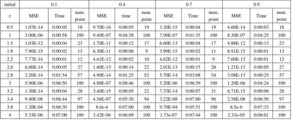
Table (3). Time and MSE of approximate solution after many training trials with uniform noise by using FFT transfer function when the variance equal to 0.05
initial 0.1 0.4 0.7 0.9
r MSE Time num.
point MSE time
num.
point MSE Time num.
point MSE Time num. point 0.5 1.07E-14 0:00:05 18 9.70E-16 0:00:05 19 3.20E-15 0:00:04 19 4.60E-14 0:00:03 18
1 3.00E-06 0:00:58 100 9.40E-07 0:04:38 100 7.90E-07 0:01:35 100 8.30E-07 0:04:25 100 1.5 1.03E-12 0:00:04 23 1.70E-11 0:00:12 17 6.60E-13 0:00:04 17 4.88E-12 0:00:13 23 1.8 7.90E-15 0:00:02 13 6.30E-11 0:00:06 9 3.99E-15 0:00:02 11 8.91E-15 0:00:01 13 2.2 7.77E-14 0:00:01 12 4.61E-12 0:00:02 10 4.62E-12 0:00:01 9 7.60E-13 0:00:01 12 2.6 6.60E-14 0:00:05 27 1.60E-13 0:00:14 22 2.01E-13 0:00:15 26 1.21E-13 0:00:05 27 2.8 3.20E-14 0:01:54 57 4.90E-14 0:01:25 52 5.70E-14 0:03:08 54 3.08E-13 0:00:25 57 3 5.90E-06 0:06:50 100 4.88E-07 0:08:46 100 5.20E-06 0:06:59 100 1.20E-06 0:04:24 100 3.2 1.30E-14 0:00:04 28 3.40E-15 0:00:05 22 7.33E-14 0:00:07 31 6.71E-15 0:00:06 28 3.4 9.40E-08 0:06:44 97 4.56E-07 0:05:30 94 3.22E-08 0:07:00 96 2.56E-08 0:06:50 97 3.8 1.20E-04 0:06:30 100 8.6e-6 0:07:00 100 9.70E-04 0:05:51 100 6.5e-6 0:07:33 100
Table (4). Time and MSE of approximate solution after many training trials with uniform noise by using tansig transfer function when the variance equal to 0.5
initial 0.1 0.4 0.7 0.9
r MSE Time num.
point MSE time
num.
point MSE Time num.
point MSE time
num. point 0.5 6.00E-03 0:01:57 18 6.95E-06 0:01:42 19 3.30E-14 0:00:25 19 5.69E-09 0:00:20 18
1 0.00388 0:01:54 100 4.98E-03 0:00:07 100 0.00313 0:01:53 100 0.0038 0:01:50 100 1.5 1.50E-13 0:00:07 23 4.79E-04 0:00:07 17 5.50E-04 0:00:11 17 3.56E-04 0:01:26 23 1.8 8.12E-06 0:01:47 13 5.39E-04 0:01:00 9 3.40E-14 0:00:06 11 3.60E-07 0:00:19 13 2.2 3.67E-13 0:00:08 12 1.05E-13 0:00:05 10 1.29E-03 0:00:09 9 5.60E-17 0:00:04 12 2.6 4.33E-03 0:00:12 27 3.08E-06 0:01:59 22 2.31E-03 0:00:20 26 4.05E-04 0:01:27 27 2.8 0.00654 0:01:18 57 0.00434 0:00:46 52 0.00503 0:01:03 54 0.00286 0:00:55 57 3 0.0071 0:02:30 100 0.00751 0:02:00 100 0.00863 0:01:55 100 0.00684 0:02:01 100 3.2 0.0262 0:00:13 28 0.0193 0:00:17 22 0.0725 0:00:25 31 0.0316 0:01:00 28 3.4 0.0296 0:00:41 97 0.0398 0:01:00 94 0.0353 0:01:03 96 0.0264 0:00:55 97 3.8 0.0507 0:02:00 100 0.0548 0:01:46 100 0.185 0:01:55 100 0.0623 0:01:59 100
4 0.073 0:01:52 100 0.055 0:01:40 100 0.081 0:01:47 100 0.0371 0:01:55 100
Table (5). Time and MSE of approximate solution after many training trials with uniform noise by using logsig transfer function when the variance equal to 0.5
initial 0.1 0.4 0.7 0.9
r MSE time num.
point MSE time
num.
point MSE Time num.
point MSE Time num. point 0.5 2.00E-03 0:00:16 18 8.10E-14 0:00:07 19 1.30E-13 0:00:13 19 1.50E-13 0:00:10 18
1 0.00615 0:00:07 100 0.00475 0:00:14 100 0.0059 0:00:06 100 0.0055 0:00:49 100 1.5 8.80E-06 0:00:50 23 7.50E-07 0:01:48 17 1.54E-06 0:02:11 17 6.59E-04 0:00:31 23 1.8 3.90E-12 0:00:07 13 1.50E-14 0:00:06 9 3.60E-07 0:00:13 11 3.54E-03 0:00:14 13 2.2 1.43E-14 0:00:11 12 7.18E-16 0:00:06 10 6.60E-04 0:00:47 9 2.40E-12 0:00:07 12 2.6 5.20E-06 0:00:38 27 3.50E-04 0:01:08 22 3.60E-04 0:01:30 26 8.80E-14 0:00:42 27 2.8 0.00217 0:01:40 57 0.00826 0:01:40 52 0.00493 0:02:00 54 0.00275 0:01:59 57 3 0.0059 0:01:40 100 0.0069 0:01:53 100 0.00185 0:02:02 100 0.0011 0:02:10 100 3.2 0.0281 0:00:13 28 0.00947 0:01:20 22 0.0126 0:00:18 31 0.0251 0:00:30 28 3.4 0.0281 0:01:20 97 0.033 0:01:50 94 0.084 0:01:44 96 0.0124 0:02:00 97 3.8 0.0526 0:00:32 100 0.056 0:00:53 100 0.0729 0:01:43 100 0.0185 0:01:58 100
4 0.0853 0:02:08 100 0.0427 0:01:53 100 0.0174 0:01:56 100 0.0395 0:02:00 100
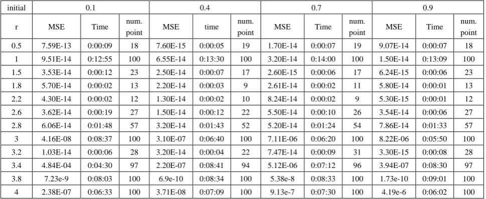
Table (6). Time and MSE of approximate solution after many training trials with uniform noise by using FFT transfer function when the variance equal to 0.5
initial 0.1 0.4 0.7 0.9
r MSE Time num.
point MSE time
num.
point MSE Time num.
point MSE Time num. point 0.5 7.59E-13 0:00:09 18 7.60E-15 0:00:05 19 1.70E-14 0:00:07 19 9.07E-14 0:00:07 18
1 9.51E-14 0:12:55 100 6.55E-14 0:13:30 100 3.20E-14 0:14:00 100 1.50E-14 0:13:09 100 1.5 3.53E-14 0:00:12 23 2.50E-14 0:00:07 17 2.60E-15 0:00:06 17 6.24E-15 0:00:06 23 1.8 5.70E-14 0:00:02 13 2.20E-14 0:00:03 9 2.61E-14 0:00:02 11 5.80E-14 0:00:01 13 2.2 4.30E-14 0:00:02 12 1.30E-14 0:00:02 10 8.24E-14 0:00:02 9 5.30E-15 0:00:01 12 2.6 3.62E-14 0:00:19 27 1.50E-14 0:00:12 22 5.50E-14 0:00:10 26 3.54E-14 0:00:06 27 2.8 6.06E-14 0:01:48 57 3.20E-14 0:01:43 52 5.20E-14 0:01:24 54 7.86E-14 0:01:33 57 3 4.16E-08 0:08:37 100 3.10E-07 0:06:40 100 7.11E-06 0:06:20 100 8.22E-06 0:05:50 100 3.2 1.03E-14 0:00:06 28 3.20E-14 0:00:04 22 7.47E-14 0:00:09 31 3.30E-15 0:00:08 28 3.4 4.84E-04 0:04:30 97 2.20E-07 0:08:41 94 5.12E-06 0:07:12 96 3.94E-07 0:08:30 97 3.8 7.23e-9 0:08:03 100 6.9e-10 0:08:34 100 5.38e-8 0:08:33 100 1.73e-10 0:09:01 100
Table (7). Time and MSE of approximate solution after many training trials with uniform noise by using logsig transfer function when the variance equal to 15
initial 0.1 0.4 0.7 0.9
r MSE time num.
point MSE time
num.
point MSE time
num.
point MSE time
num. point 0.5 1.83 0:30:07 18 2.13 0:44:01 19 1.04 0:33:09 19 4.03 0:23:20 18 1.5 3.56 0:17:00 23 1.004 0:18:08 17 1.52 0:28:10 17 3.54 0:45:01 23 1.8 1.65 0:05:03 13 4.41 0:04:12 9 3.85 0:03:44 11 1.94 0:05:07 13 2.2 82.3 0:06:05 12 32.5 0:04:06 10 22.9 0:06:09 9 2.74 0:03:02 12 2.6 284 0:04:04 27 320 0:09:01 22 23.4 0:12:07 26 53.7 0:17:01 27 3.2 179 0:05:05 28 177 0:04:12 22 231 0:03:56 31 324 0:04:03 28
Table (8). Time and MSE of approximate solution after many training trials with uniform noise by using tansig transfer function when the variance equal to 15
initial 0.1 0.4 0.7 0.9
r MSE time num.
point MSE time
num.
point MSE time
num.
point MSE time
num. point 0.5 1.19 0:17:53 18 1.63 0:33:40 19 2.72 0:40:00 19 3.51 0:20:09 18 1.5 2.97 0:16:07 23 1.63 0:25:09 17 3.52 0:40:12 17 1.84 0:38:08 23 1.8 2.08 0:04:48 13 4.85 0:04:07 9 6.11 0:07:10 11 3.24 0:05:09 13 2.6 8.55 0:05:00 27 5.31 0:10:00 22 9.67 0:04:40 26 2.83 0:12:01 27 3.2 522 0:04:31 28 441 0:05:48 22 303 0:08:09 31 261 0:07:03 28
Table (9). Time and MSE of approximate solution after many training trials with uniform noise by using FFT transfer function when the variance equal to 15
initial 0.1 0.4 0.7 0.9
r MSE time num.
point MSE time
num.
point MSE Time num.
point MSE time
num. point 0.5 1.30E-04 1:05:18 18 1.27E-07 0:01:11 19 2.31E-06 0:30:20 19 4.62E-05 0:40:04 18 1.5 5.80E-08 0:09:31 23 4.28E-09 0:17:09 17 9.22E-07 0:10:08 17 1.06E-08 0:22:03 23 1.8 2.78E-08 0:01:30 13 7.42E-10 0:00:59 9 8.32E-10 0:00:05 11 3.16E-08 0:01:03 13 2.2 4.60E-09 0:00:14 12 1.50E-09 0:00:09 10 2.01E-08 0:00:39 9 2.40E-08 0:01:01 12 2.6 8.00E-08 0:10:44 27 3.23E-07 0:14:03 22 2.73E-06 0:17:10 26 2.20E-08 0:11:04 27 3.2 6.89E-07 0:04:20 28 3.20E-07 0:06:02 22 5.21E-06 0:03:55 31 6.16E-07 0:05:12 28
4.6. Training for Case with Normal Noise
We train case with normal noise and variances 0.05, 0.5 and 15. Table from (10) to (18) contain the results.
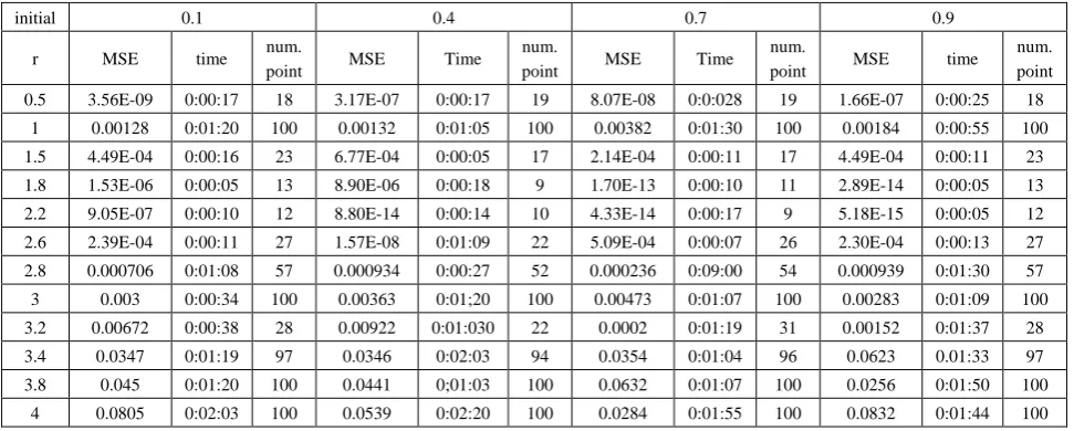
Table (10). Time and MSE of approximate solution after many training trials with normal noise by using logsig transfer function when the variance equal to 0.05
initial 0.1 0.4 0.7 0.9
r MSE time num.
point MSE Time
num.
point MSE Time num.
point MSE time
num. point 0.5 3.56E-09 0:00:17 18 3.17E-07 0:00:17 19 8.07E-08 0:0:028 19 1.66E-07 0:00:25 18
1 0.00128 0:01:20 100 0.00132 0:01:05 100 0.00382 0:01:30 100 0.00184 0:00:55 100 1.5 4.49E-04 0:00:16 23 6.77E-04 0:00:05 17 2.14E-04 0:00:11 17 4.49E-04 0:00:11 23 1.8 1.53E-06 0:00:05 13 8.90E-06 0:00:18 9 1.70E-13 0:00:10 11 2.89E-14 0:00:05 13 2.2 9.05E-07 0:00:10 12 8.80E-14 0:00:14 10 4.33E-14 0:00:17 9 5.18E-15 0:00:05 12 2.6 2.39E-04 0:00:11 27 1.57E-08 0:01:09 22 5.09E-04 0:00:07 26 2.30E-04 0:00:13 27 2.8 0.000706 0:01:08 57 0.000934 0:00:27 52 0.000236 0:09:00 54 0.000939 0:01:30 57 3 0.003 0:00:34 100 0.00363 0:01;20 100 0.00473 0:01:07 100 0.00283 0:01:09 100 3.2 0.00672 0:00:38 28 0.00922 0:01:030 22 0.0002 0:01:19 31 0.00152 0:01:37 28 3.4 0.0347 0:01:19 97 0.0346 0:02:03 94 0.0354 0:01:04 96 0.0623 0.01:33 97 3.8 0.045 0:01:20 100 0.0441 0;01:03 100 0.0632 0:01:07 100 0.0256 0:01:50 100
Table (11). Time and MSE of approximate solution after many training trials with normal noise by using tansig transfer function when the variance equal to 0.05
initial 0.1 0.4 0.7 0.9
R MSE Time num.
point MSE Time num.
point MSE Time num.
point MSE Time num. point 0.5 2.08E-07 0:01:40 18 3.24E-08 0:01:02 19 2.22E-06 0:00:59 19 8.13E-05 0:01:03 18
1 2.03E-06 0:01:22 100 1.70E-03 0:15:05 100 1.60E-03 0:05:09 100 0.00125 0:08:03 100 1.5 2.26E-07 0:00:18 23 4.89E-04 0:01:02 17 7.79E-14 0:00:13 17 2.02E-04 0:00:20 23 1.8 9.66E-06 0:00:06 13 9.89E-10 0:00:13 9 1.70E-04 0:00:04 11 8.33E-06 0:00:16 13 2.2 4.07E-06 0:00:09 12 1.40E-04 0:00:10 10 9.66E-06 0:00:06 9 1.78E-04 0:00:15 12 2.6 1.59E-03 0:00:13 27 3.44E-04 0:00:24 22 1.19E-03 0:00:16 26 1.81E-04 0:01:30 27 2.8 3.67E-04 0:02:59 57 2.19E-03 0:00:04 52 9.24E-04 0:00:32 54 7.11E-04 0:02:01 57 3 0.00118 0:05:38 100 0.00194 0:00:40 100 0.00322 0:04:55 100 0.00184 0:03:46 100 3.2 1.13E-02 0:00:31 28 1.44E-02 0:00:13 22 9.97E-04 0:00:38 31 8.20E-03 0:01:05 28 3.4 0.0328 0:00:11 97 0.0275 0:00:10 94 0.0283 0:01:08 96 0.0384 0:02:04 97 3.8 0.0533 0:01:02 100 0.0583 0:00:07 100 0.0423 0:00:08 100 0.0593 0:00:10 100
4 0.0926 0:00:05 100 0.0488 0:01:50 100 0.0964 0:01:00 100 0.0375 0:00:40 100
Table (12). Time and MSE of approximate solution after many training trials with normal noise by using FFT transfer function when the variance equal to 0.05
initial 0.1 0.4 0.7 0.9
r MSE Time num.
point MSE Time
num.
point MSE Time
num.
point MSE Time
num. point 0.5 1.18E-13 0:00:09 18 1.49E-13 0:00:05 19 1.40E-13 0:00:04 19 5.60E-15 0:00:03 18
1 6.68E-06 0:07:03 100 5.09E-06 0:08:17 100 3.08E-06 0:06:09 100 1.78E-07 0:07:29 100 1.5 1.72E-13 0:00:06 23 3.51E-11 0:00:10 17 5.56E-13 0:00:02 17 1.03E-13 0:00:02 23 1.8 8.53E-14 0:00:03 13 3.71E-13 0:00:05 9 1.07E-12 0:00:05 11 1.41E-12 0:00:01 13 2.2 3.06E-13 0:00:03 12 2.43E-12 0:00:03 10 2.61E-12 0:00:04 9 2.30E-13 0:00:03 12 2.6 5.07E-14 0:00:05 27 6.52E-14 0:00:08 22 2.48E-14 0:00:06 26 8.90E-14 0:00:06 27 2.8 5.20E-14 0:01:03 57 6.49E-14 0:01:23 52 2.21E-13 0:01:04 54 2.85E-14 0:01:51 57 3 8.27E-04 0:01:55 100 4.95E-04 0:07:02 100 1.93E-07 0:11:01 100 4.59E-07 0:10:08 100 3.2 5.65E-14 0:00:17 28 2.19E-15 0:00:14 22 4.01E-14 0:00:04 31 4.82E-15 0:00:04 28 3.4 9.92E-14 0:17:51 97 9.99E-14 0:14:13 94 9.69E-14 0:06:12 96 7.85E-14 0:08:05 97 3.8 1.00E-13 0:31:33 100 6.65E-14 0:29:08 100 1.75E-14 0:33:01 100 6.83E-14 0:40:02 100
4 7.90E-04 0:07:30 100 3.20E-08 1:08:00 100 4.81e-7 0:45:08 100 1.63e-7 0:33:04 100
Table (13). Time and MSE of approximate solution after many training trials with normal noise by using logsig transfer function when the variance equal to 0.5
initial 0.1 0.4 0.7 0.9
r MSE Time num.
point MSE Time num.
point MSE Time num.
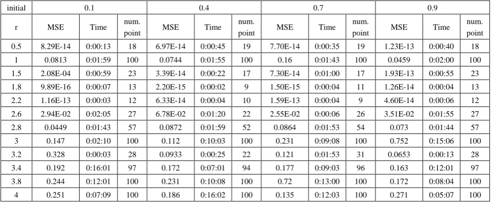
point MSE Time num. point 0.5 8.29E-14 0:00:13 18 6.97E-14 0:00:45 19 7.70E-14 0:00:35 19 1.23E-13 0:00:40 18
1 0.0813 0:01:59 100 0.0744 0:01:55 100 0.16 0:01:43 100 0.0459 0:02:00 100 1.5 2.08E-04 0:00:59 23 3.39E-14 0:00:22 17 7.30E-14 0:01:00 17 1.93E-13 0:00:55 23 1.8 9.89E-16 0:00:07 13 2.20E-15 0:00:02 9 1.50E-15 0:00:04 11 1.26E-14 0:00:04 13 2.2 1.16E-13 0:00:03 12 6.33E-14 0:00:04 10 1.59E-13 0:00:04 9 4.60E-14 0:00:06 12 2.6 2.94E-02 0:02:05 27 6.78E-02 0:01:20 22 2.55E-02 0:00:06 26 3.51E-02 0:01:55 27 2.8 0.0449 0:01:43 57 0.0872 0:01:59 52 0.0864 0:01:53 54 0.073 0:01:44 57 3 0.147 0:02:10 100 0.112 0:10:03 100 0.231 0:09:08 100 0.752 0:15:06 100 3.2 0.328 0:00:03 28 0.0933 0:00:25 22 0.121 0:01:53 31 0.0653 0:00:13 28 3.4 0.192 0:16:01 97 0.172 0:07:01 94 0.177 0:09:03 96 0.163 0:12:01 97 3.8 0.244 0:12:01 100 0.231 0:10:08 100 0.72 0:13:00 100 0.172 0:08:04 100
Table (14). Time and MSE of approximate solution after many training trials with normal noise by using tansig transfer function when the variance equal to 0.5
initial 0.1 0.4 0.7 0.9
r MSE Time num.
point MSE time num.
point MSE time num.
point MSE Time num. point 0.5 3.03E-17 0:00:06 18 8.12E-15 0:00:05 19 4.68E-14 0:00:13 19 9.80E-15 0:00:06 18
1 1.04E-01 0:00:36 100 9.27E-02 0:02:01 100 1.13E-01 0:01:45 100 0.179 0:01:50 100 1.5 2.18E-14 0:00:09 23 6.67E-14 0:00:06 17 2.31E-15 0:00:08 17 4.47E-13 0:00:09 23 1.8 1.62E-14 0:00:03 13 2.13E-14 0:00:02 9 2.00E-06 0:00:11 11 3.91E-14 0:00:04 13 2.2 1.36E-13 0:00:04 12 4.04E-15 0:00:02 10 2.77E-13 0:00:03 9 3.60E-14 0:00:01 12 2.6 1.80E-14 0:00:09 27 2.71E-14 0:00:49 22 6.08E-02 0:00:55 26 6.90E-03 0:10:15 27 2.8 0.0808 0:01:40 57 0.0428 0:01:50 52 0.0351 0:01:55 54 0.0572 0:01:33 57 3 0.116 0:00:43 100 0.18 0:01:18 100 0.155 0:11:01 100 0.127 0:08:07 100 3.2 0.243 0:00:20 28 0.0714 0:00:31 22 0.274 0:00:09 31 0.0219 0:00:10 28 3.4 0.156 0:05:52 97 0.281 0:10:08 94 0.912 0:13:02 96 0.271 0:08:01 97 3.8 0.125 0:012:07 100 0.612 0:16:00 100 0.163 0:09:06 100 0.731 0:07:05 100
4 0.312 0:10:07 100 0.717 0:06:08 100 0.813 0:08:02 100 0.936 0:05:10 100
Table (15). Time and MSE of approximate solution after many training trials with normal noise by using FFT transfer function when the variance equal to 0.5
initial 0.1 0.4 0.7 0.9
r MSE Time num.
point MSE Time num.
point MSE time
num.
point MSE Time
num. point 0.5 8.70E-15 0:00:02 18 5.75E-15 0:00:02 19 2.30E-15 0:00:02 19 1.74E-15 0:00:02 18
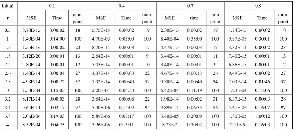
1 1.40E-04 0:14:00 100 4.70E-03 0:05:00 100 8.40E-04 0:35:00 100 9.37E-03 0:30:01 100 1.5 1.55E-16 0:00:02 23 8.70E-14 0:00:03 17 4.47E-15 0:00:03 17 3.32E-14 0:00:02 23 1.8 3.12E-20 0:00:01 13 2.64E-14 0:00:01 9 3.44E-14 0:00:01 11 7.40E-15 0:00:01 13 2.2 7.80E-14 0:00:01 12 5.03E-14 0:00:01 10 3.40E-14 0:00:01 9 6.86E-15 0:00:01 12 2.6 1.40E-14 0:00:04 27 4.37E-14 0:00:03 22 4.67E-14 0:00:13 26 9.49E-14 0:00:02 27 2.8 4.93E-14 0:00:22 57 7.92E-14 0:00:49 52 9.30E-14 0:00:40 54 2.03E-14 0:01:46 57 3 1.53E-04 0:15:05 100 2.20E-04 0:04:53 100 6.42E-04 0:11:49 100 1.24E-04 0:13:06 100 3.2 8.17E-14 0:00:03 28 3.64E-14 0:00:06 22 1.98E-14 0:00:02 31 8.37E-15 0:00:03 28 3.4 9.64E-14 0:02:17 97 5.40E-06 0:14:09 94 9.89E-14 0:06:33 96 5.61E-06 0:16:07 97 3.8 2.06E-06 0:19:03 100 5.89E-06 0:07:17 100 3.40E-05 0:20:09 100 1.80E-05 1:00:12 100
4 8.52E-04 0:04:25 100 3.26E-06 0:15:11 100 8.23e-7 0:30:02 100 2.11e-5 0:16:03 100
Table (16). Time and MSE of approximate solution after many training trials with normal noise by using logsig transfer function when the variance equal to 15
Initial 0.1 0.4 0.7 0.9
r MSE time num.
point MSE Time
num.
point MSE time
num.
point MSE Time
Table (17). Time and MSE of approximate solution after many training trials with normal noise by using tansig transfer function when the variance equal to 15
initial 0.1 0.4 0.7 0.9
r MSE time num.
point MSE Time
num.
point MSE Time
num.
point MSE Time
num. point 0.5 69.6 1:03:00 18 36.3 0:30:01 19 9.22 0:50:01 19 10.3 0:55:03 18 1.5 47.2 0:50:08 23 23.9 1:05:00 17 73.8 0:30:08 17 16.5 0:44:07 23 1.8 102 1:05:01 13 25.2 0:30:01 9 22.2 0:40:07 11 102.2 0:32:05 13 2.2 14.3 0:16:01 12 20.3 0:31:00 10 23.5 0:45:01 9 25.9 0:20:02 12 2.6 15.2 0:23:12 27 44.2 0:15:04 22 63.9 0:12:07 26 72.9 0:12:02 27 3.2 11.8 1:02:00 28 24.3 0:43:01 22 9.22 1:12:02 31 12.3 0:37:08 28
Table (18). Time and MSE of approximate solution after many training trials with normal noise by using FFT transfer function when the variance equal to 15
initial 0.1 0.4 0.7 0.9
r MSE Time num.
point MSE Time
num.
point MSE Time
num.
point MSE time
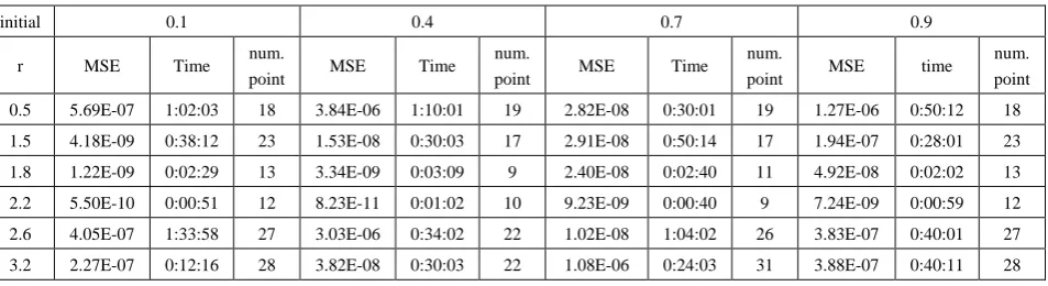
num. point 0.5 5.69E-07 1:02:03 18 3.84E-06 1:10:01 19 2.82E-08 0:30:01 19 1.27E-06 0:50:12 18 1.5 4.18E-09 0:38:12 23 1.53E-08 0:30:03 17 2.91E-08 0:50:14 17 1.94E-07 0:28:01 23 1.8 1.22E-09 0:02:29 13 3.34E-09 0:03:09 9 2.40E-08 0:02:40 11 4.92E-08 0:02:02 13 2.2 5.50E-10 0:00:51 12 8.23E-11 0:01:02 10 9.23E-09 0:00:40 9 7.24E-09 0:00:59 12 2.6 4.05E-07 1:33:58 27 3.03E-06 0:34:02 22 1.02E-08 1:04:02 26 3.83E-07 0:40:01 27 3.2 2.27E-07 0:12:16 28 3.82E-08 0:30:03 22 1.08E-06 0:24:03 31 3.88E-07 0:40:11 28
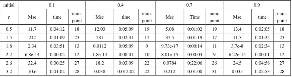
4.7. Training for Case with Logistic Noise
We train case with logistic noise and variances 0.05, 0.5 and 15. Table (19) to (27) contains the results.
Table (19). Time and MSE of approximate solution after many training trials with logistic noise by using logsig transfer function when the variance equal to 0.05
initial 0.1 0.4 0.7 0.9
r Mse time num.
point Mse time
num.
point Mse time
num.
point Mse Time
num. point 0.5 1.11E-13 0:00:18 18 1.16E-13 0:00:10 19 3.98E-10 0:00:12 19 3.16E-14 0:00:13 18
1 0.000691 0:00:53 100 0.000872 0:01:35 100 0.000186 0:03:09 100 0.000186 0:04:44 100 1.5 2.03E-14 0:00:20 23 1.25E-13 0:00:11 17 2.98E-10 0:14:00 17 4.93E-12 0:013:09 23 1.8 2.78E-13 0:00:08 13 1.99E-12 0:00:07 9 7.89E-06 0:00:06 11 1.38E-16 0:00:17 13 2.2 6.23E-07 0:00:07 12 4.90E-13 0:00:08 10 1.69E-07 0:00:38 9 1.20E-14 0:00:05 12 2.6 1.37E-03 0:00:05 27 5.87E-04 0:00:03 22 8.81E-06 0:00:17 26 2.60E-04 0:00:21 27 2.8 0.000732 0:00:21 57 0.000912 0:00:40 52 0.000830 0:00:12 54 0.00143 0:00:10 57 3 0.00323 0:00:22 100 0.00133 0:00:16 100 0.00265 0:06:51 100 0.00356 0:05:34 100 3.2 0.0097 0:00:30 28 0.00841 0:05:04 22 0.00956 0:00:11 31 0.00432 0:00:16 28 3.4 0.0203 0:01:19 97 0.0563 0:12:07 94 0.0164 0:06:03 96 0.0132 0:04:23 97 3.8 0.0417 0:05:01 100 0.0237 0:04:03 100 0.0638 0:03:09 100 0.0385 0:03:02 100
Table (20). Time and MSE of approximate solution after many training trials with logistic noise by using tansig transfer function when the variance equal to 0.05
initial 0.1 0.4 0.7 0.9
R Mse time num.
point Mse time
num.
point Mse Time num.
point Mse time
num. point 0.5 2.42E-07 0:00:34 18 6.77E-14 0:00:43 19 2.07E-13 0:00:27 19 4.01E-14 0:00:23 18
1 0.000649 0:00:29 100 9.50E-04 0:06:55 100 1.82E-04 0:50:03 100 0.000134 0:07:23 100 1.5 2.65E-14 0:00:10 23 1.17E-05 0:00:30 17 2.35E-06 0:00:19 17 7.07E-12 0:01:11 23 1.8 1.53E-06 0:00:36 13 2.48E-13 0:00:03 9 1.80E-14 0:00:10 11 1.52E-12 0:00:07 13 2.2 6.20E-06 0:00:05 12 1.69E-07 0:00:18 10 1.70E-07 0:00:14 9 1.33E-12 0:00:02 12 2.6 7.03E-04 0:00:15 27 3.70E-04 0:00:05 22 1.80E-06 0:02:05 26 2.68E-04 0:00:31 27 2.8 0.00028 0:04:18 57 0.00128 0:04:03 52 0.000309 0:03:02 54 0.000503 0:00:13 57 3 0.00137 0:04:03 100 0.00217 0:01:39 100 0.00186 0:07:23 100 0.00697 0:04:45 100 3.2 5.77E-03 0:00:30 28 6.36E-03 0:05:09 22 8.72E-03 0:00:25 31 9.58E-03 0:04:56 28 3.4 0.0260 0:03:35 97 0.0313 0:01:30 94 0.0342 0:04:08 96 0.0283 0:05:03 97 3.8 0.0604 0:30:02 100 0.0608 0:01:09 100 0.058 0:02:04 100 0.093 0:02:34 100
4 0.0459 0:01:39 100 0.096 0:03:05 100 0.0681 0:01:39 100 0.0853 0:01:25 100
Table (21). Time and MSE of approximate solution after many training trials with logistic noise by using FFT transfer function when the variance equal to 0.05
initial 0.1 0.4 0.7 0.9
R Mse time num.
point Mse Time
num.
point Mse Time num.
point Mse time
num. point 0.5 1.17E-13 0:00:08 18 3.38E-13 0:00:04 19 1.81E-13 0:00:06 19 3.44E-16 0:00:04 18
1 2.65E-06 0:04:30 100 9.89E-14 0:11:15 100 7.33E-06 0:06:25 100 2.57E-08 0:15:46 100 1.5 9.79E-13 0:00:03 23 1.73E-12 0:00:06 17 1.59E-12 0:00:07 17 1.36E-13 0:00:04 23 1.8 1.89E-12 0:00:02 13 6.67E-12 0:00:02 9 1.97E-13 0:00:02 11 3.87E-13 0:00:01 13 2.2 5.05E-13 0:00:00 12 4.91E-13 0:00:01 10 3.68E-12 0:00:03 9 2.18E-14 0:00:01 12 2.6 4.37E-14 0:00:14 27 2.95E-13 0:00:08 22 3.95E-12 0:00:07 26 1.63E-13 0:00:08 27 2.8 1.49E-11 0:01:23 57 7.68E-14 0:01:27 52 7.60E-14 0:01:17 54 2.05E-04 0:01:38 57 3 2.99E-07 0:14:03 100 1.02E-06 0:12:32 100 2.98E-07 0:22:02 100 1.94E-06 0:10:29 100 3.2 1.84E-14 0:00:05 28 8.30E-14 0:00:17 22 6.89E-14 0:00:06 31 5.03E-15 0:00:08 28 3.4 1.82E-06 0:11:23 97 1.55E-07 0:09:57 94 5.47E-06 0:08:35 96 2.93E-07 0:15:34 97 3.8 3.09E-04 0:07:16 100 9.92E-04 0:10:23 100 1.23E-04 0:10:11 100 2.83E-04 0:08:23 100
4 3.51E-07 0:25:42 100 4.31E-14 0:03:32 100 1.09e-6 0:06:50 100 3.97e-8 0:15:57 100
Table (22). Time and MSE of approximate solution after many training trials with logistic noise by using logsig transfer function when the variance equal to 0.5
Initial 0.1 0.4 0.7 0.9
R Mse time num.
point Mse time num.
point Mse Time
num.
point Mse time num. point 0.5 3.60E-03 0:00:30 18 5.87E-03 0:00:21 19 1.99E-03 0:00:08 19 4.04E-15 0:00:06 18
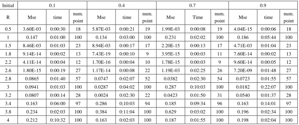
1 0.147 0:01:00 100 0.134 0:03:00 100 0.231 0:02:02 100 0.186 0:05:44 100 1.5 8.46E-03 0:01:03 23 8.94E-03 0:00:17 17 2.20E-15 0:00:13 17 4.71E-03 0:01:04 23 1.8 9.14E-14 0:00:02 13 7.43E-19 0:00:10 9 3.95E-15 0:00:03 11 7.60E-14 0:00:02 13 2.2 4.11E-14 0:00:04 12 1.70E-16 0:00:04 10 1.78E-15 0:00:03 9 9.60E-14 0:00:05 12 2.6 1.80E-15 0:00:19 27 1.17E-14 0:00:08 22 1.19E-03 0:02:25 26 7.20E-09 0:01:48 27 2.8 0.0865 0:01:40 57 0.0747 0:02:07 52 0.0382 0:02:30 54 0.0723 0:01:55 57 3 0.0941 0:01:03 100 0.0287 0:04:02 100 0.287 0:10:03 100 0.0182 0:22:07 100 3.2 0.0807 0:00:14 28 0.0024 0:02:30 22 0.0423 0:01:50 31 0.0540 0:01:37 28 3.4 0.163 0:06:00 97 0.286 0;10:03 94 0.185 0:09:34 96 0.163 0:14:01 97 3.8 0.234 0:02:03 100 0.384 0:11:04 100 0.629 0:03:02 100 0.196 0:02:34 100
Table (23). Time and MSE of approximate solution after many training trials with logistic noise by using tansig transfer function when the variance equal to 0.5
initial 0.1 0.4 0.7 0.9
r Mse Time num.
point Mse time
num.
point Mse Time num.
point Mse time
num. point 0.5 1.70E-14 0:00:11 18 9.80E-06 0:00:07 19 3.83E-16 0:00:08 19 8.08E-14 0:00:11 18
1 0.0424 0:01:20 100 1.24E-01 0:20:02 100 2.73E-01 0:10:03 100 0.376 0:12:04 100 1.5 7.20E-04 0:00:16 23 3.68E-06 0:00:12 17 5.80E-15 0:00:11 17 3.49E-06 0:02:30 23 1.8 4.50E-17 0:00:04 13 5.39E-16 0:00:02 9 9.08E-16 0:00:03 11 2.14E-17 0:00:04 13 2.2 4.71E-15 0:00:02 12 1.31E-15 0:00:03 10 9.58E-15 0:00:07 9 3.60E-14 0:00:03 12 2.6 4.30E-03 0:01:02 27 6.89E-03 0:00:17 22 3.36E-02 0:04:44 26 3.91E-02 0:00:40 27 2.8 0.0691 0:01:30 57 0.0387 0:02:03 52 0.723 0:02:01 54 0.083 0:01:54 57 3 0.0762 0:01:23 100 1.03 0:02:21 100 0.09877 0:12:02 100 0.367 0:03:20 100 3.2 0.0234 0:00:45 28 0.0945 0:00:06 22 0.0307 0:00:07 31 0.0167 0:00:42 28 3.4 0111 0:02:09 97 0.382 0:12:32 94 0.938 0:16:02 96 0.738 0:09:03 97 3.8 131 0:01:08 100 0.171 0:15:00 100 0.629 0:12:07 100 0.282 0;10:01 100
4 0.163 0:02:04 100 0.273 0:10:23 100 0.739 0:12:34 100 0.864 0:14:52 100
Table (24). Time and MSE of approximate solution after many training trials with logistic noise by using FFT transfer function when the variance equal to 0.5
initial 0.1 0.4 0.7 0.9
r Mse Time num.
point Mse time
num.
point Mse Time num.
point Mse time
num. point 0.5 2.70E-15 0:00:02 18 1.11E-16 0:00:02 19 1.30E-15 0:00:03 19 7.60E-14 0:00:02 18
1 4.16E-06 0:10:14 100 1.30E-03 0:06:47 100 5.25E-04 0:25:33 100 4.86E-04 0:033:01 100 1.5 3.30E-16 0:00:05 23 7.30E-14 0:00:01 17 1.30E-14 0:00:02 17 1.20E-15 0:00:02 23 1.8 4.22E-14 0:00:01 13 1.70E-14 0:00:01 9 4.36E-17 0:00:01 11 6.30E-14 0:00:01 13 2.2 9.93E-15 0:00:01 12 3.31E-15 0:00:01 10 1.80E-14 0:00:01 9 4.80E-14 0:00:01 12 2.6 1.00E-14 0:00:05 27 7.92E-14 0:00:04 22 4.74E-15 0:00:10 26 4.04E-14 0:00:03 27 2.8 5.25E-14 0:00:43 57 7.47E-15 0:00:27 52 1.98E-16 0:00:50 54 1.05E-15 0:00:33 57 3 2.30E-04 0:04:05 100 7.51E-04 0:06:48 100 3.82E-04 0:05:00 100 3.42E-06 0:10:30 100 3.2 9.88E-15 0:00:04 28 7.93E-15 0:00:02 22 1.65E-14 0:00:02 31 9.16E-15 0:00:03 28 3.4 2.92E-12 0:40:03 97 9.14E-14 0:04:06 94 1.00E-13 1:00:41 96 2.98E-13 1:02:20 97 3.8 6.40E-15 0:02:15 100 8.32E-14 0:20:43 100 7.07E-14 0:22:10 100 9.28E-14 0:10:28 100
4 9.98E-14 0:15:16 100 6.24E-04 0:15:09 100 4.04e-8 0:18:20 100 3.82e-9 0:19:01 100
Table (25). Time and MSE of approximate solution after many training trials with logistic noise by using logsig transfer function when the variance equal to 15
initial 0.1 0.4 0.7 0.9
r Mse time num.
point Mse time
num.
point Mse Time num.
Table (26). Time and MSE of approximate solution after many training trials with logistic noise by using tansig transfer function when the variance equal to 15
initial 0.1 0.4 0.7 0.9
r Mse Time num.
point Mse time
num.
point Mse Time
num.
point Mse time
num. point 0.5 7.55 0:01:36 18 25.8 0:02:09 19 16.5 0:03:01 19 1.44 0:02:23 18 1.5 46.3 0:01:04 23 5.10 0:01:04 17 2.92 0:03:22 17 1.98 0:04:10 23 1.8 1.39e-14 0:00:07 13 1.05e-15 0:00:10 9 9.7e-15 0:00:01 11 6.40e-14 0:00:02 13 2.2 4.8e-14 0:00:10 12 2.93e-13 0:02;10 10 1.09e-14 0:01:04 9 2.95e-14 0:02:03 12 2.6 12.6 0:00:17 27 21.5 0:02:01 22 2.01 0:03:33 26 0.238 0:23:53 27 3.2 0.245 0:00:14 28 0.132 0:01:01 22 0.0453 0:09:12 31 0.743 0:03:04 28
Table (27). Time and MSE of approximate solution after many training trials with logistic noise by using FFT transfer function when the variance equal to 15
initial 0.1 0.4 0.7 0.9
r Mse Time num.
point Mse time
num.
point Mse Time num.
point Mse time
num. point 0.5 1.80E-15 0:00:02 18 2.19E-15 0:00:02 19 1.26E-16 0:00:02 19 1.93E-15 0:00:02 18 1.5 3.18E-14 0:00:02 23 2.80E-15 0:00:02 17 1.97E-16 0:00:03 17 7.30E-15 0:00:02 23 1.8 7.01E-16 0:00:01 13 3.30E-16 0:00:01 9 2.20E-16 0:00:02 11 3.20E-15 0:00:02 13 2.2 1.40E-15 0:00:02 12 3.80E-15 0:00:01 10 3.16E-15 0:00:01 9 1.83E-15 0:00:01 12 2.6 3.82E-09 0:01:09 27 3.40E-14 0:00:06 22 4.23E-15 0:00:09 26 8.23E-14 0:00:07 27 3.2 1.80E-07 0:06:01 28 2.92E-06 0:07:03 22 2.23E-08 0:12:02 31 1.09E-08 0:17:10 28
![Figure 1. Bifurcation diagram of the Logistic map [26]](https://thumb-us.123doks.com/thumbv2/123dok_us/8713709.1741848/3.595.318.548.284.413/figure-bifurcation-diagram-logistic-map.webp)