A Combined Motif Discovery Method

University of New Orleans University of New Orleans

ScholarWorks@UNO

ScholarWorks@UNO

University of New Orleans Theses and

Dissertations Dissertations and Theses

8-6-2009

A Combined Motif Discovery Method

A Combined Motif Discovery Method

Daming Lu

University of New Orleans

Follow this and additional works at: https://scholarworks.uno.edu/td

Recommended Citation Recommended Citation

Lu, Daming, "A Combined Motif Discovery Method" (2009). University of New Orleans Theses and Dissertations. 990.

https://scholarworks.uno.edu/td/990

This Thesis is protected by copyright and/or related rights. It has been brought to you by ScholarWorks@UNO with permission from the rights-holder(s). You are free to use this Thesis in any way that is permitted by the copyright and related rights legislation that applies to your use. For other uses you need to obtain permission from the rights-holder(s) directly, unless additional rights are indicated by a Creative Commons license in the record and/or on the work itself.

A Combined Motif Discovery Method

A Thesis

Submitted to the Graduate Faculty of the University of New Orleans

in partial fulfillment of the requirements for the degree of

Master of Science in

Computer Science Bioinformatics

by

Daming Lu

B.E. Dalian University of Technology, 2007

ii

Acknowledgment

I would like to express my great gratitude to Dr. Stephen Winters-Hilt. As my

advisor, he has helped me tremendously to understand the importance of academic

research. He gave me the enthusiasm to begin research in the field of Bioinformatics,

which I previously did not know anything about. I aspire to keep this enthusiasm in the

future endeavors, as he has after years of research. His intelligence and accomplishments

make him an excellent mentor yet he still knows how to balance work and fun.

iii

Table of Contents

Chapter 1 Introduction ...1

Chapter 2 Gibbs Sampling ...2

Chapter 3 Simulated Tempering ...9

Chapter 4 Mutual Information ...18

Chapter 5 Method and Result ...29

Chapter 6 Conclusion and Discussion ...34

References ...36

Appendix A.1 Gibbs Sampling Source Code in PERL ...40

A.2 Simulated Tempering Code in C++ ...45

A.3 Mutual Information Source Code in PERL ...51

A.4 Motif Discovery via Mutual Information ...54

iv

List of Illustrations

Fig 2.1

Gibbs Sampling Algorithm Sketch

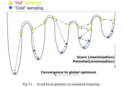
Fig 3.1 Avoid local optimum via simulated tempering

Fig 3.2

TLC 5 = 0.50, 0.62, 0.74, 0.86, 0.98

Fig 5.1

Method flowchart

v

Abstract

A central problem in the bioinformatics is to find the binding sites for regulatory motifs.

This is a challenging problem that leads us to a platform to apply a variety of data mining

methods.

In the efforts described here, a combined motif discovery method that uses mutual

information and Gibbs sampling was developed. A new scoring schema was introduced

with mutual information and joint information content involved. Simulated tempering

was embedded into classic Gibbs sampling to avoid local optima.

This method was applied to the 18 pieces DNA sequences containing CRP binding sites

validated by Stormo and the results were compared with Bioprospector. Based on the

results, the new scoring schema can get over the defect that the basic model PWM only

contains single positioin information. Simulated tempering proved to be an adaptive

adjustment of the search strategy and showed a much increased resistance to local

optima.

Keywords:

Transcription Factor Binding Site Gibbs Sampling

Mutual Information Information Content Simulated Tempering

1

Chapter 1 Introduction

Uncovering the hidden mechanism of gene transcription control is a huge effort in the

post genomic era. Various methods have been invented to decipher the information

encoded in DNA sequences. The approaches come from two ways: the biological

experimental way or computational biology way.

Biology experiment is accurate in locating the functional DNA subsequences in the

genome sequences, but is time and labour consuming. Conversely, the computational way

is high throughput and time saving, but needs a large amount of DNA sequences as

prerequisite and is not very accurate.

Motif discovery by computer programs, however, became feasible as the publicly

available biosequences databases grow in site and high performance computers become

cheaply available. Consequently, many fundamental computational methods to discover

functional biosequences have been developed. Those methods include the Gibbs

sampling method introduced by Lawrence [1] and EM method used by Elkan [2].

Although these methods achieve some degree of success, and many computer programs

have been developed based on them, the problem of motif discovery from DNA

sequences still remains difficult because of its complex nature.

In addition, the search strategy differs largely also. Some basic algorithms like consensus

[3], EM [4] and Gibbs sampler [5] brought solutions to this problem, but the result was

not satisfactory enough. The enhanced computer programs based on them such as MEME

[6], AlignAce [7], and Bioprospector [8] are more powerful in dealing with true data,

since these programs are enhanced by using more complex models and considering more

parameters. After considering the above algorithms, we found a varied Gibbs sampling

method similar to Bioprospector with some advantages. A new scoring schema was

introduced with further incorporation of a novel mutual information motif finder to

strengthen the overall method. Simulated tempering was also embedded into classic

2

Chapter 2 Gibbs Sampling

Gibbs sampling is a Markov chain Monte Carlo method for joint distribution estimation

when the full conditional distributions of all the relevant random variables are available.

The Gibbs sampling procedure iteratively draws samples from the full conditional

distributions. The samples collected in this way are guaranteed to converge to the true

joint distribution as long as there is no zero-probability in the target joint distribution.

Gibbs sampling strategy has been applied to Bayesian hierarchical models in

bioinformatics. The first introduction of the methodology is its application to the motif

discovering problem in DNA sequence analysis [5].

This chapter serves as a brief review for the applications of Gibbs sampling in the field of

bioinformatics. The working mechanism of Gibbs sampling was discussed and some

essential concepts needed for understanding this method was introduced.

2.1 Introduction to Gibbs Sampling

Gibbs sampling is a technique to draw samples from a join distribution based on the full

conditional distributions of all the associated random variables. Though the idea goes

back to the work of Hasting (1970) [9], whose focus was on its Markov chain Monte

Carlo (MCMC) nature, the Gibbs sampler was first formally introduced by Geman and

Geman [10] to the field of image processing. The work caught the attention of the

statistics society (especially boosted by the thesis of Gelfand and Smith (1992) [11]).

Since then, the applications of Gibbs sampling have covered both the Bayesian world and

the world of classical statistics. In the former case, Gibbs sampling is often used to

estimate posterior distributions, and in the latter, it is often applied to likelihood

estimation [12]. In particular, Gibbs sampling has become a popular alternative to the

3

context, where the associated random variables of interest include both the hidden

variables (i.e., the missing data) and the parameters of the model that describe the

complete data.

To provide answers to this type of questions, EM is a numerical maximization procedure

that climbs in the likelihood landscape aiming to find the model parameters and the

hidden variables that maximize the likelihood function. In contrast, Gibbs sampling

provides the means to estimate the target joint distribution of the hidden variables and the

model parameters as a whole, and leave the estimation of the random variables for later

(i.e. after the samples are drawn), where maximum a posterior (MAP) estimates are often

used. Thus, Gibbs sampling suffers less from the problem of local maxima than EM. This

property makes Gibbs sampling a suitable candidate for solving the model-based

problems in bioinformatics, where the likelihood function usually consists of a large

amount of modes due to the high complexity of the data.

In the remainder of this chapter, the applications of Gibbs sampling to the hierarchical

Bayesian models were shown that address an important problem in systems biology. The

goal is to discover regulation mechanism of genes. A typical framework by means of

computational biology for this kind of study is composed of two steps. In the first step groups of genes that share similar expression profiles (which measured by the microarray

technology) are found. (These genes are called to be coexpressed). This is done by

performing clustering algorithms to the gene expression profiles (i.e., microarray data).

The second step is based on the general assumption that coexpression implies

coregulation. For each group of genes found in the first step, the DNA sequences that are

related to the regulation of these genes are extracted and common patterns of these

sequences (called motifs) are seeked. The positions of these conserved motifs are likely

to be the binding sites of transcription factors, which are the executors of the gene

regulation mechanism. We show in this thesis that the Gibbs sampling strategy can be

applied to both the motif finding problem of DNA sequences and other bioinformatics

4

We will first review the working mechanism of Gibbs sampling. Then some basic

biological concepts for understanding the biological problems of interest are introduced.

2.2 Explanation in Mathematical Terms

2.2.1 Parameters

The first requirement for the Gibbs sampling is the observable data. The observed data

will be denoted Y. In the general case of the Gibbs sampling, the observed data remains

constant throughout. Gibbs sampling requires a vector of parameters of interest that are

initially unknown.

These parameters will be denoted by the vector Φ. Nuisance parameters, Θ, are also

initially unknown. The goal of Gibbs sampling is to find estimates for the parameters of

interest in order to determine how well the observable data fits the model of interest, and

also whether or not data independent of the observed data fits the model described by the

observed data. Gibbs sampling requires an initial starting point for the parameters. In our

situation, this is set randomly. Then, one at a time, a value for each parameter of interest

is sampled given values for the other parameters and data.

Once all of the parameters of interest have been sampled, the nuisance parameters are

sampled given the parameters of interest and the observed data. At this point, the process

is started over. The power of Gibbs sampling is that the joint distribution of the

parameters will converge to the joint probability of the parameters given the observed

data.

The Gibbs sampler requires a random starting point of parameters of interest, Φ, and nuisance parameters, Θ, with observed data Y, from which a converging distribution can

5 (₁(0),(0)₂ ,...,(0)_D ,(0)),

Steps a-d are then repeatedly run.

a) Sample ₁( 1)i from p( ₁| ₂( )i ,..., ( )_Di , ( )i , )Y

b) Sample ₂( 1)i from p( ₂| ₁( 1)i ,( )₃i ,..., ( )_Di , ( )i , )Y

…… ……

c) Sample ( 1)_Di from p( _D| ₁( 1)i ,...,( 1)_Di₁,( )i, )Y

d) Sample( 1)i from p( | ( 1)₁i ,...,( 1)_Di , )Y

2.2.2 ParametersMultiple Alignments

One application of Gibbs sampling useful in computational molecular biology is the

detection and alignment of locally conserved regions (motifs) in sequences of amino

acids or nucleic acids assuming no prior information in the patterns or motifs. Gibbs

sampling strategies claim to be fast and sensitive, avoiding the problem that EM

algorithms fall into as far as getting trapped by local optima.

2.3 Algorithm Scheme

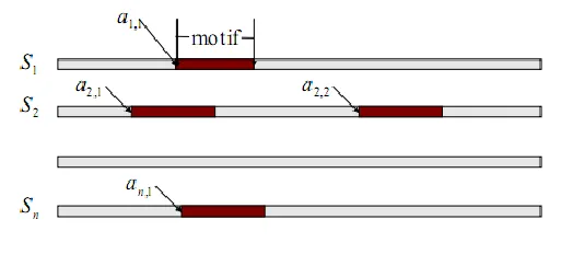
First the basic multiple alignment strategy is examined where a single motif is desired.

The most basic implementation, known as a site sampler, assumes that there is exactly

one motif element located within each sequence.

2.3.1 Notation

• N: number of sequences • S₁...S_n: set of sequences

• W: width of motif to be found in the sequences

6

• c_{i j k, ,} : Observed counts of residue j in position i of motif k . j ranges from 1…J. i

ranges from 0..W where c_0,j contains the counts of residue j in the background. If it is assumed that only a single motif is searched for, the k term can drop out.

• q_{i j,} : frequency of residue j occurring in position i of the motif. i ranges from 0..W as above.

• a_k: vector of starting positions of the motifs within the sequences. k ranges from 1. .N . • b_j: pseudocounts for each residue – needed according to Bayesian statistical rules to eliminate problems with zero counts.

• B : The total number of pseudocounts. _j j

B



b .

2.3.2 Initialization

Once the sequences are known, the counts for each residue can calculated. Initially, c_0,j

will contain the total counts of residue j within all of the sequences andc_{i j,} is initialized to 0 for all other values of i. This is a summary observed data. The site sampler is then

initialized by randomly selecting a position for the motif within each sequence and

recording these positions ina_k. The counts are updated according to this initial alignment. After the observed counts are set,q_{i j,} can be calculated.

, ,

1

i j j

i j

c

b

q

N

B





 

Equation 1: Motif Residue Frequencies

, 0,

0, 1

o j j

j j

k k

c

b

q

c

B











7

2.3.3 Predictive Update Step

The first step, known as the predictive update step, selects one of the sequences and

places the motif within that sequence in the background and updates the residue counts.

One of the N sequences, z, is chosen. The motif in sequence z is taken from the model

and placed in the background. The observed counts c_{i j,} are updated as are the frequenciesq_{i j,} . The selection of z can be random or in a specified order.

2.3.4 Sampling Step

In the sampling step, a new motif position for the selected sequence is determined by

sampling according to a weight distribution. All of the possible segments of width W.

within sequence z are considered. For each of these segments x, a weight A_x is

calculated according to the ratio x x

x

Q A

P

 where _,

1

i W

x i r i

Q q







is the model residue

frequency according to equation 1 if segment x is in the motif model, and _0, 1 i W x r i P q 





is

the background residue frequency according to equation 2. r_i refers to the residue located at position i of segment x . Once A_xis calculated for every possible x, a new position a_z is chosen by randomly sampling over the set of weights A_x. Thus, possible starting positions with higher weights will be more likely to be chosen as the new motif

position than those positions with lower weights. Since this is a stochastic process, the

starting position with the highest weight is not guaranteed to be chosen. Once the

iterative predictive update and sampling steps have been performed for all of the

sequences, a probable alignment is present. For this alignment, a maximum posteriori

(MAP) estimate can be calculated using equation 3:

, ,

1 1 0,

log

W J

i j i j

i j j

q

F

c

q

 





8

2.3.5 Explanation

The idea is that the more accurate the predictive update step is, the more accurate the

sampling step will be since the background will be more distinguished from the motif

description. Given random positions a_kin the sampling step, the pattern description q_{i j,}

will not favor any particular segment. Once some correct a_k have been selected by chance, theq_{i j,} begins to favor a particular motif.

globalMaxAlignmentProb = 0 For Iteration = 1 to N

Initialize Random alignment localMaxAlignmentProb = 0; while (not in local maximum

and

innerloop < MAXLOOP) do

for each sequence do{ Predictive Update Sample

}

calculate AlignmentProb if(AlignmentProb

>localMaxAlignmentProb){

localMaxAlignmentProb=AlignmentProb; not in local maximum=true; }

Innerloop++; }

If(localMaxAlignmentProb ==globalMaxAlignmentProb) exit -> max found twice

else if (localMaxAlignmentProb >

globalMaxAlignmentProb)

globalMaxAlignmentProb=

localMaxAlignmentProb }

9

Chapter 3 Simulated Tempering

3.1 Simulated Annealing

Simulated annealing is a generalization of a Monte Carlo method for examining the

equations of state and frozen states of n-body systems [13]. The concept is based on the

manner in which liquids freeze or metals recrystalize in the process of annealing. In an

annealing process a melt, initially at high temperature and disordered, is slowly cooled so

that the system at any time is approximately in thermodynamic equilibrium. As cooling

proceeds, the system becomes more ordered and approaches a "frozen" ground state at

T=0. Hence the process can be thought of as an adiabatic approach to the lowest energy

state. If the initial temperature of the system is too low or cooling is done insufficiently

slowly the system may become quenched forming defects or freezing out in metastable

states (ie. trapped in a local minimum energy state).

The original Metropolis scheme was that an initial state of a thermodynamic system was

chosen at energy E and temperature T, holding T constant the initial configuration is perturbed and the change in energy dE is computed. If the change in energy is negative the new configuration is accepted. If the change in energy is positive it is accepted with a

probability given by the Boltzmann factor exp -(dE/T). This processes is then repeated sufficient times to give good sampling statistics for the current temperature, and then the

temperature is decremented and the entire process repeated until a frozen state is

achieved at T=0.

By analogy the generalization of this Monte Carlo approach to combinatorial problems is

straightforward [14, 15]. The current state of the thermodynamic system is analogous to

the current solution to the combinatorial problem, the energy equation for the

thermodynamic system is analogous to at the objective function, and ground state is

analogous to the global minimum. The major difficulty (art) in implementation of the

algorithm is that there is no obvious analogy for the temperature T with respect to a free

10

minima (quenching) is dependent on the "annealing schedule", the choice of initial

temperature, how many iterations are performed at each temperature, and how much the

temperature is decremented at each step as cooling proceeds.

There are certain optimization problems that become unmanageable using combinatorial

methods as the number of objects becomes large. A typical example is the traveling

salesman problem, which belongs to the NP-complete class of problems. For these

problems, there is a very effective practical algorithm called simulated annealing (thus

named because it mimics the process undergone by misplaced atoms in a metal when it’s

heated and then slowly cooled). While this technique is unlikely to find the optimum

solution, it can often find a very good solution, even in the presence of noisy data.

The traveling salesman problem can be used as an example application of simulated

annealing. In this problem, a salesman must visit some large number of cities while

minimizing the total mileage traveled. If the salesman starts with a random itinerary, he

can then pairwise trade the order of visits to cities, hoping to reduce the mileage with

each exchange. The difficulty with this approach is that while it rapidly finds a local

minimum, it cannot get from there to the global minimum.

Simulated annealing improves this strategy through the introduction of two tricks. The

first is the so-called "Metropolis algorithm" [16], in which some trades that do not lower

the mileage are accepted when they serve to allow the solver to "explore" more of the

possible space of solutions. Such "bad" trades are allowed using the criterion that

/

(0,1)

D T

e





R

where Dis the change of distance implied by the trade (negative for a "good" trade;

positive for a "bad" trade), T is a "synthetic temperature," and R(0,1)is a random number in the interval

 

0,1 . _D is called a "cost function," and corresponds to the free energy in the case of annealing a metal (in which case the temperature parameter would actually be

11

absolute temperature scale). If T is large, many "bad" trades are accepted, and a large part of solution space is accessed. Objects to be traded are generally chosen randomly, though

more sophisticated techniques can be used.

The second trick is, again by analogy with annealing of a metal, to lower the

"temperature." After making many trades and observing that the cost function declines

only slowly, one lowers the temperature, and thus limits the size of allowed "bad" trades.

After lowering the temperature several times to a low value, one may then "quench" the

process by accepting only "good" trades in order to find the local minimum of the cost

function. There are various "annealing schedules" for lowering the temperature, but the

results are generally not very sensitive to the details.

There is another faster strategy called threshold acceptance [17]. In this strategy, all good

trades are accepted, as are any bad trades that raise the cost function by less than a fixed

threshold. The threshold is then periodically lowered, just as the temperature is lowered

in annealing. This eliminates exponentiation and random number generation in the

Boltzmann criterion. As a result, this approach can be faster in computer simulations.

12

3.2 Simulated Tempering

To alleviate the vulnerability of Gibbs sampling to local optima trapping, we propose to

combine a thermodynamic method, called simulated tempering, with Gibbs sampling.

The combined method was validated using synthetic data and actual promoter sequences

extracted from CRP binding site of E.Coli. It is noteworthy that the marked improvement of the efficiency presented here is attributable solely to the improvement of the search

method.

Simulated tempering is an accelerated version of simulated annealing and has two main

features. First, the temperature of the system is continuously adjusted during the

optimization process and may be increased as well as decreased. Second, the adjustment

of temperature is performed without detailed analysis of the potential landscape.

Temperature control is performed by introducing a second Markov chain.

In this section, we demonstrate that simulated tempering (ST) [18], which is one of many

proposals from the field of thermodynamics for the systematic avoidance of local optima

in multivariate optimization problems, is quite useful for reducing the vulnerability of

Gibbs sampling to local optima. The application of ST to a genetics problem has already

been reported [19]. SA and potential deformation [20,21], which has already succeeded

in other problems of bioinformatics, are also rooted in the field of thermodynamics. ST

and SA employ a temperature parameter T, the introduction of which into a local alignment problem has already been reported [22].

The novelty of ST is that it attempts to adjust the value of adaptively to the current score

of alignments. By changing T, ST adopts continuously changing search methods ranging

from a fast deterministic-like search to a random-like search, reducing the possibility of

being trapped in local optima. This principal is schematically shown in Fig. 1. In the

present work, we implemented and tested an ST-enhanced Gibbs sampling algorithm for

TFBS discovery, which we call GibbsST. The validation of our algorithm is also

13

14

3.3 Gibbs Sampling with Simulated Tempering

3.3.1 Gibbs sampling with temperature

In this section, we introduce a temperature, T, into the "classic" Gibbs sampling

algorithm proposed by Lawrence et al. The details of the algorithm (row selection order,

pseudocount, etc.) will be introduced later along with the implementation of our

algorithm. For simplicity, it is assumed that all N of input sequences have exactly one occurrence (the OOPS-model) of the pattern, which is always W_m bp long, and negative strands are not considered.

The algorithm holds a current local alignment, A, and a current PWM (Position Weight Matrix),q_{i j,} , which are iteratively updated as a Markov chain until the convergence to a pattern. The alignment A is represented by the starting points of aligned segments,x_k, which form a gapless sequence block. The first half of an iterative step is the

recalculation of elements of the current PWM according to the current alignment,

excluding the k-th row. Then in the second half of a step, the k-th row of the current

alignment is updated by sampling a new value of x_kaccording to weights derived from

, i j

q . Let l(1), l(2), ... denote the entire sequence of the row to be updated. We set the

probability of the new starting point being x proportional to ( x) , 1/ x Q T P  _{ } where 1 ( ), 0 m W

x l x i i i

Q q



 





is the likelihood that the x-th substring

(x ~ x - 1 + W_m-th letters) of the k-th input sequence comes from the probabilistic

model represented by the current PWM, and

1

( ) 0

m

W

x l x i

i

P p



 





is the likelihood that the

same subsequence comes from a totally random sequence of the base composition

observed for the entire input,

p

_0,1,2,3 (that is,

p

_{G A C T, , ,} ). The T is a positive value which is the "temperature" of the system. Note that the computational complexity of the single

15

It is easy to see that the above introduced iteration step maximizes 1

( ), ( ) 0

( / )

m W

l x i i l x i i

q p 



 





unless T is extremely large. Since k circulates all N of input sequences, this is a maximization of 



q_{i j,} log(q_{i j,} / p_i) after all. Hence, the Gibbs sampling introduced here has the relative entropy of the pattern PWM against the background

model as its objective-function (or score) to be maximized, and so does our algorithm.

Following the convention of statistical physics, however, we refer to TFBS discovery as a

minimization of the potential U, which is currently (negative relative entropy). Because

we are not proposing a new definition of U, we do not evaluate the sensitivity and

specificity of our new algorithm. In principle, the sensitivity and specificity must be

independent from the search method in the limit of large step number.

When T = ß = 1, the method is reduced to the classic Gibbs sampling without the idea of

temperature. In this case, there always is a finite probability of selection of non-optimal

x, which gives rise to the escape from the local minima. However, the magnitude of the

escape probability may not be sufficient for deep local minima, because the probability is

ultimately limited by the pseudocount. The temperature strongly affects the behavior of

the optimization algorithm. It is easy to see that when T is large enough, the x selection is

almost random (T → ∞ means that the probabilities of all x are 1), and the algorithm is

very inefficient despite the high immunity to the local minima problem. When T → 0, on

the other hand, a very quick convergence to local minima only results, because the

movement in the solution space is a "steepest-descent" movement. In simulated

annealing, the temperature is initially set to an ideally large value,T_h, where essentially no barrier exists in the potential landscape, and then slowly lowered. There is a

theoretical guarantee that SA converges to the global minimum when the temperature

decreases slowly enough [23]. However, it is frequently unrealistic to follow the theory

16

3.3.2 Temperature scheduling

Simulated tempering is an accelerated version of simulated annealing and has two main

features. First, the temperature of the system is continuously adjusted during the

optimization process and may be increased as well as decreased. Second, the adjustment

of temperature is performed without detailed analysis of the potential landscape.

Temperature control is performed by introducing a second Markov chain (i.e. a random

walk along the temperature axis) that is coupled with U.

In simulated tempering, the temperature of the system takes one of the N_T temperature levels, _{0 1 2}... ₁

T N

T  T T T _ (usually, it is required that ₁~ T

N h

T _ T ).During the optimization, the temperature is updated accordingly to the transition rates, R, given by a Metropolis-Hastings-like formula:

1

1

(

)

1/ (1

)

(

)

/ (1

)

i i

i i

R T

T

S

R T

T

S

S

 

  













where S_ is given by

1 1

exp(

)

exp(

)

i i i i

U

T

Z

U

T

Z

 





i

Z is a normalizing factor usually called the partition function of the system, defined as

exp( ). i i U Z T 





How should the temperature levels be decided in ST? Unlike the case of simulated

17

parameters of simulated tempering, except for the requirement of small temperature

intervals. According to the equations above, the equilibrium distributions of U defined for

neighboring values of T_i must be overlapped to ensure finite transition rates between these temperature levels. This mainly requires small temperature intervals.

The temperature levels must be decided empirically, which leaves us a vast combination

of T_i to explore. However, considering the success of classic Gibbs sampling (and our preliminary test, whose data are not shown), we can safely assume that T_h1 for the current problem.

Moreover, a good starting point has already been pointed out by Frith et al. [7]. In their

thesis, they introduced temperature in a manner similar to ours, and reported that a slight

improvement of performance was observed only when they fixed the temperature to

slightly lower than 1.

So, in this thesis, we chose the result from their work.

18

Chapter 4 Mutual Information & Joint Information

4.1 Mutual Information

The concept of entropy is very important in information theory. It is characterized by the

quantity of a random process’ uncertainty. If the entropy of the source is less than the

capacity of the channel, then asymptotically error free communication can be achieved.

The entropy of a discrete random variable X with a frequency p(x) is defined by:

2

( ) ( ) log ( )

x

H X  



p x p x

The joint entropy of two discrete random variables X and Y with frequency p(x) and p(y),

respectively, is defined by:

2 ,

( , ) ( , ) log ( , )

x y

H X Y  



p x y p x y

Conditional entropy H (X|Y) is the entropy of a random variable X, given another

random variable Y, which is def ined by:

2 ,

( | ) ( , ) log ( | )

x y

H X Y  



p x y p x y

The relative entropy D(p||q) is a measure of the distance between two distributions. The relative entropy (or Kullback Leibler distance) between two frequency p(x) and q(x) is

defined as

2

( ) ( || ) ( ) log

( )

p x

D p q p x

q x

19

The relative entropy is always non-negative and is zero if and only if p = q. However, it is

not a true distance between distributions since it is not symmetric and does not satisfythe

triangle inequality.

The reduction in uncertainty X due to the knowledge of random variable Y is called the

mutual information. For two random variables X and Y, this reduction is:

2 ,

( , )

( ; )

( , ) log

( ) ( )

x y

p x y

I X Y

p x y

p x p y





Where p(x, y) is the joint frequency, p(x) and p(y) are marginal frequency of x and y,

respectively, and I(X; Y) is a measure of the dependence between the two random

variables. It is symmetric in X and Y and is always non-negative.

Therefore, a recursive style mutual information concept was proposed. The main purpose

is to capture more information given more joint frequency. Thus, for a third random

variable Z, the accumulative mutual information is defined as:

2

, ,

( , , )

( , ; )

( , , )log

( , ) ( )

x y z

p x y z

I X Y Z

p x y z

p x y p z





The meaning of accumulative mutual information is that given a single random varable

and joint frequency of a group of random varables, it can calculate the intense of linkage

20

4.2 Scoring Schema

As mentioned in previous section, one of the important problems in motif discovery area

is finding the known TFBSs in a given DNA sequence or promoter region (known motif

prediction). In this section we focus on this problem and at first, some definitions and

notations further used in this thesis are introduced.

Let N { , , , }A C G T be the four nucleotide letters' of which DNA sequences are

composed. We have the DNA sequence Dd₁,...,d_n(a promoter region) onN , and let us suppose that we have t known TFBSs of the length l which are represented by a matrix

t l

B_ for a given TF, and we intend to investigate by B, where D possesses a motif instance or transcription factor binding site corresponding to the given TF. For finding

the position of this motif instance inD, we first create a position weight matrix W of B, and then we scan all subsequences Rd_i,...,d_{i l 1} for i1,...,n l 1 of D, and align position weight matrix W with each R. All the subsequences which score is greater than a cutoff are reported as motif instances. The creation of position weight matrix W from TFBSs and calculating the score of alignment W with a subsequence are called scoring schema.

The accuracy of the solution in this search problem depends on how we design the

scoring schema, and how the position weight matrix is constructed. In this section we

first discuss two existing scoring schemas which are employed for ranking known motifs

and predicting TFBSs, later a new scoring schema is presented.

4.2.1 Independent scoring schema

The first scoring schema is a conventional method and is employed in many theses. In

this scoring schema, it is assumed that all positions in a given motif are completely

21

Suppose we have a promoter region D and a TFBS matrix B of some known motifs. Assume that F b j( , ) (bN and1 j l) shows the occurrences of nucleotide b in

column j of the matrix B. Employing this function, a frequency P is made as follows:

( , )

( , ) F b j ( ) 1 ,

P b j a b b N j l

t

     

where a b( ) is the smoothing parameter (a b( ) 0.01 ). Later, a position weight matrix

4 l

W_ is made as follows:

,

( , )

log 1 ,

( )

b j

P b j

W b N j l

p b

    

where each p b( ) shows the occurrence frequency of nucleotide b(independent of

nucleotides in the other position) in a random sequence (obviously p b( )0.25 for every

bN ).

Now, let Rbe a DNA subsequence with the length l of a promoter region D (

1,..., l

Rr r and r_iN for 1 i l). For computing the score of R, we align position weight matrix W with Rand calculate Score R₁( ) as follows:

_{1 ,} 1 ( ) i l r i i

Score R W







This score can be normalized as follows:

1 1

1

1 1

( )

( ) Score R MinScore ,

NScore R

MaxScore MinScore 





where MaxScore₁ and MinScore₁ are calculated as follows:

1 , 1 max{ }, l b j b N j MaxScore W  





and _{1 ,}

22

4.2.2 Dependent scoring schema

The second scoring schema was first introduced in [24]. In this scoring schema,

dependency between some positions in a given TFBS is assumed. This method uses a

statistical approach to find dependent positions in a set of known TFBSs. Therefore, if the

dependent positions of a set of TFBSs are available, then this scoring schema is defined

as follows.

Similar to the previous definition, we have a promoter region D and t binding sites of the length l which are represented by a matrix B_{t l} for a given TF. Also, assume that

1 1

([ ,..., _m],[ ,..., _m])

F b b j j shows the occurrences of bases b₁,...,b b_m( _iN for1 i m) in dependent positions j₁,..., j_m in the matrix B(positions j₁,...,j_m are determined by statistical approaches [24]). As an example, F A C A T([ , , , ],[3, 4,8,11]) represents the

number of occurrences of A, C, A, and T in the positions 3, 4, 8, and 11 in a given matrix

B. It should be noted that the positions j₁,..., j_m are dependent and not necessarily consecutive.

The corrected frequency for the bases b₁,...,b_min positions j₁,...,j_m is defined as:

1 1

1 1 1

([ ,...,

],[ ,...,

])

([ ,...,

],[ ,...,

])

m m

( ,...,

),

m m m

F b

b

j

j

P b

b

j

j

a b

b

t





where a b( ,...,₁ b_m)is a smoothing parameter and can be calculated as follows:

1 1

( ,..., _m) ( ) ... ( _m).

a b b a b  a b

Now, the position weight matrix W corresponding to the binding sites is calculated as:

1 1

1 1

[ ,..., ],[ ,..., ] 2

1

([ ,...,

],[ ,...,

])

log

( ) ... (

)

m m

m m

b b j j

m

P b

b

j

j

W

p b

p b



23

Finally, for a given subsequence Rr₁,...,r_l (r_iNand 1 i l) of D, we align position weight matrix W with R and calculate Score R₂( ) as follows:

1 2

1 1

1 1

2 [ ],[ ] [ , ],[ , ] [ ,..., ],[ , ... , ]

1 1 1

( )

...

m

j_i i j_i j_i i i j_i j_{i m} i i m

k

k k

r j r r j j r r j j

i i i

Score R

W

W

W

  

  

  









 



where k₁ is the number of independent positions, k₂ is the number of dependent

positions order 2 (nucleotides at positions j_i and j_i₁) and km the number of dependent positions order m (nucleotides at positions j j_i, _i1,...,j_{i m 1}).

The normalized version of Score R₂( )can be defined as:

2 2

2

2 2

( )

( )

Score R

MinScore

,

NScore R

MaxScore

MinScore







where MaxScore₂ and MinScore₂can be calculated as follows:

1 2

1 2 , 1 1 ,...,

1 2 1

2 , [ , ],[ ] [ ,..., ],[ ]

[ , ] ( ) [ ,..., ] ( ... )

1 1 1

max

max

...

max

m

i i i m i i m

m

k

k k

b j b b j j b b j j

b N b b N N b b N N

i i i

MaxScore

W

W

_

W

_

     

  









 



and

1 2

1 2 , 1 1 ,...,

1 2 1

2 , [ , ],[ ] [ ,..., ],[ ]

[ , ] ( ) [ ,..., ] ( ... )

1 1 1

min

min

...

min

m

i i i m i i m

m

k

k k

b j b b j j b b j j

b N b b N N b b N N

i i i

MinScore

W

W

_

W

_

     

  

24

4.2.3 New scoring schema

In the previous subsections we presented two scoring schemas. In the first, nucleotides in

all positions in a given TFBS are considered as independent, but this may not be true in

all cases because it is shown that dependency between some positions are important

[25,26]. In the second, dependency between some positions in a TFBS are considered,

but this model has also two problems: first, calculation of dependency between positions

is sophisticated, and second, final score is obtained by summation of all the scorings

obtained by each order dependent positions, which are not in the same range.

As mentioned, all positions in TFBSs may be dependent, because the length of TFBSs are

short, therefore all positions in TFBS may be involved in the interaction with a factor and

dependency between all positions are important. TFBSs are short regions in promoter

region that TFs can be bonded to them to provide initial conditions for gene transcription.

By mutual comparison of TFBS corresponding to a specific TF, we see that some

positions in TFBS are mutated and some other ones are conserved.

Since the length of a TFBS is short, therefore it seems that both mutated and conserved

positions play an important role in binding of TF and TFBS. During a transcription

process, TFBS region constructs structure by hydrogen bonds and this causes the

attraction of TF to this region. Thus, with respect to the above feature of this process, it

seems that the conserved positions and mutated positions cause this attraction. Also, with

respect to that, the average specific free energy of binding to all binding sites play an

important role in this attraction, and by considering that this energy is directly related to

the information content of the preferred binding sites [26], we use the information content

for TFBS scoring. We also illustrate the original motif discovering via mutual

25

Similar to the previous subsection, suppose that we have a promoter region D and binding site matrix B_{t l} for a given TF. Employing information theory, we compute the information content (IC) of a set of TFBSs which are represented by the matrix B with position independency as follows:

1

( , ) ( , ) log ,

( )

l

j b N

F b j F b j IC

t t p b

 







where F and p are computed similar to independent scoring schema. From this formula, we have 0IC2l. Now, we assume that positions are mutually dependent, and F b b([ , ],[ ,_{1 2} j j_{1 2}])shows the number of the occurrence of nucleotides b₁ and b₂in positions j₁ and j₂ in the given matrix B. As an example, P A T([ , ],[3,8]) represents the frequency of the occurrence of the pair A and T in the positions 3 and 8 in a given

matrix B. Clearly, the number of all two combinations of four nucleotides is equal to 16, and the number of all two combinations of l tuples is equal to l l( 1) / 2. In this case, the

joint information content (JIC) is computed as:

1 2

1

1 2 1 2

1 1 1 2

([ , ],[ , ]) ([ , ],[ , ]) log

( ) ( ) l l

j k j b N b N

F b b j k F b b j k JIC

t t p b p b



    



 

   

,

and for this formula we have 0JIC 4l.

Obviously, we get more information from JIC when the positions are more conserved.

Now, the problem is to add up the information of the mutated positions to JIC which have

not been considered yet. For this reason, we compute the mutual information (MI) as

follows:

1 2

1

1 2 1 2

1 1 1 2

([ , ],[ , ]) ([ , ],[ , ]) log

( , ) ( , ) l l

j k j b N b N

F b b j k F b b j k MI

t t F b j F b k



    



 

26

and from this formula we have 0MI 2l . The relation of MI and JIC for each position pairs is as follows. If MI = 0 then JIC = 4 and consequently MI + JIC = 4, if MI = 2 then

JIC = 2 and consequently MI + JIC = 4. This condition implies that JIC does show less

information and by adding up MI we can get more information. Actually MI carries

meaningful information that can not be discarded. On the other hand, IC = 2 means,

conservation is low but dependency between positions is high.

With regard to the above discussion, the frequency of the bases b₁ and b₂ in positions j₁

and j₂ can be defined as:

1 2 1 2

1 2 1 2 1 2

([ , ],[ , ])

([ , ],[ , ]) F b b j j ( , )

P b b j j a b b

t

  ,

where a b b( ,_{1 2}) is a smoothing parameter and can be calculated as:

1 2 1 2

( , )

( )

( )

a b b



a b



a b

,

Now, for our scoring schema, we make a position weight matrix W_{16 (( ( 1))/2)  l l} whose each entry shows the number of occurrences of a pair of nucleotides in a pair of positions. This

matrix is defined as:

1 2 1 2

1 2 1 2 1 2 1 2

[ , ],[ , ]

1 2 1 1 2 2

([ , ],[ , ]) ([ , ],[ , ])

log log

( ) ( ) ( , ) ( , )

b b j j

P b b j j P b b j j W

p b p b p b j p b j

 

  ,

where [ , ] (b b_{1 2}  N N ), 1 j j₁, ₂l and j₁  j₂.

27 1 2

1 2

1 2 1

1

3 [ , ],[ , ]

1 1

( )

j j

l l

r r j j

j j j

Score R

W



  



 

.

The normalized version of Score R₃( )can be defined as:

3 3

3

3 3

( )

( ) Score R MinScore

NScore R

MaxScore MinScore

 

 ,

where MaxScore₃ and MinScore₃are formulated as follows:

1 2 1 2

1 2

1 2 1

1

3 [ , ],[ , ]

[ , ] ( )

1 1

max { }

l l

b b j j b b N N

j j j

MaxScore W       

 

, and

1 2 1 2

1 2

1 2 1

1

3 [ , ],[ , ]

[ , ] ( )

1 1

min { }

l l

b b j j b b N N

j j j

MinScore W



    



 

.

4.3 Relative Entropy

And Relative entropy is applied as the current score of the alignments when simulated

tempering attempts to adjust the temperatur T adaptively.

log( i)

i i i p RL p q 



Relative entropy is a non-symmetric measure of the difference between two frequency

distributions P and Q. Relative entropy measures the expected number of extra bits required to code samples from P when using a code based on Q, rather than using a code based on P.

28

In our method, P represents the current alignment matrix whereas Q represents the background model. Relative entropy is also called the Kullback-Leibler distance,

meaning how different the current alignment matrix is from the background matrix. If

i i

p q , RL=0, meaning there is no difference. In our case, we are search the high relative entropy, which means the current alignment matrix is quite different from the

29

Chapter 5 Method and Result

In this chapter, a combind motif discovery method was described in detail and its result

compared with another motif finding method --- Bioprospector, follows.

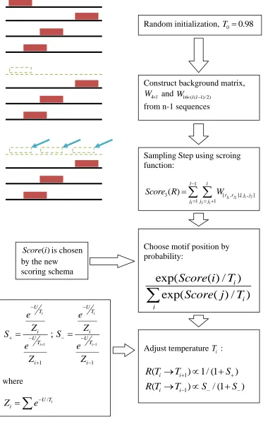
5.1 Method Sketch

The novelty of Simulated Tempering is that it attempts to adjust the value of T adaptively to the current score of alignments. The multivariate 4-nomial distribution matrix W_{N l}

was then constructed. The trick is to try to match the relative entropy of the current W_{N l}

to different temperature levels. If the current status is stable, suggesting a common motif

is captured in most sequences, and then the relative entropy of this current alignment

matrix will be high. Based on this, we tune the temperature low for a quick convergence.

If the current status is unstable, suggesting no difference between current matrix and

matrix generated from background, then the relative entropy of this current alignment

matrix will be low. Based on this, we tune the temperature high for an almost-random

search for next step.

By changing T, Simulated Tempering adopts continuously changing search methods ranging from a fast deterministic-like search to a random-like search, reducing the

possibility of being trapped in local optima. A brief flowchart about the mechanism

30

Random initialization, T₀ 0.98

Construct background matrix,

4l

W and W16 ( (l l1)/2) from n-1 sequences

Sampling Step using scroing function:

1 2

1 2

1 2 1

1

3 [ , ],[ , ]

1 1

( )

j j l l

r r j j j j j

Score R W



  



 

Choose motif position by probability:

exp(

( ) /

)

exp(

( ) /

)

i

i j

Score i

T

Score j

T



( )

Score i is chosen by the new

scoring schema

Adjust temperature T_i :

1

1

(

)

1/ (1

)

(

)

/ (1

)

i i

i i

R T

T

S

R T

T

S

S

    













1 1 1 1

;

i i i i U U T T i i U U T T i i

e

e

Z

Z

S

S

e

e

Z

Z

         





where / i U T i

Z





e



31

5.2 Testing Data

According to the above steps, a motif discovery program was developed. The test data

used was a set of DNA sequences comprising CRP binding site. CRP is a protein of

E.coli; it takes an important role in metabolism by combining to special DNA sequences

and forming DNA-protein complex which regulates some gene transcription. Stormo has

collected 18 pieces of DNA sequence; all of them have the ability to combine to CRP.

The location of the binding site in each DNA sequences was validated by experiments

(Stormo and Hartzell, 1989).

The consensus sequence is TGTGAnnnnnnTCACA; the length is 16. In order to simulate

the true situation that some sequences have no motif instance, we have added two

computer generated sequences according to a background base distribution. Altogether

there are 20 sequences to form the data set, and each sequence is at the length of 105bp.

Then we used these data serving as input data to perform the discovery.

32

5.3 Result

Our combined method, as well as Bioprospector, was run on the same testing data.

Results are shown below:

The table listed the locations and the found motifs in each sequence, altogether there are

18 sequences identified motifs. The program did not found any motif instances from the

two artificial sequences (not listed in the table). Actually, there are 24 motifs in this data

set, and the program found out 23 copies where of which 21 copies are true motif. There

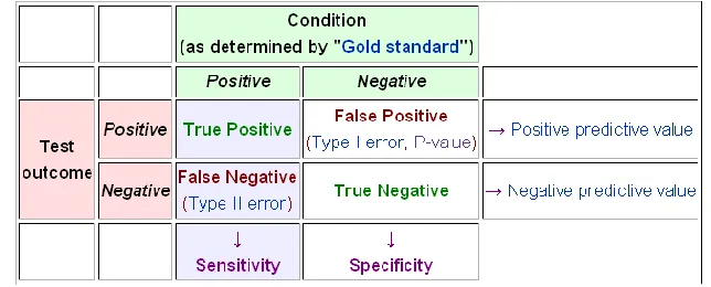
are also 2 false positives and 3 true negatives.

The Sensitivity Se TP

TP FN



 = 0.87, Specificity p

TP S

TP FP



 = 0.91. The defination

of Sensitivity and Specificity is shown in Fig 5.4

Table 5.1 Results from testing data

33

To make comparison, we used other programs to discover motifs from the same data set.

The first program used is Bioprospector (Liu et al., 2001), the service is at

http://bioprospector.stanford.edu. This program discovered 23 motifs, of which 12 motifs

are exactly matches and 12 are missed. The sensitivity and specificity of this program are

34

Chapter 6 Conclusion and Discussion

This thesis brought out a combined method to discover conserved TFBS motif of

functional DNA sequences. The combined method is a mixture of a new scoring schema

with mutual information and joint information content involved. It gets over the defect

that the basic PWM model only contained either single position information or just

neighbourhood base information. In addition, a varied Gibbs sampling algorithm with

simulated tempering embedded was employed as the discover algorithm. This algorithm

suits the situation of DNA sequence comprised no copy or multiple copies of motif (Fig ).

Through the analysis of a set of CRP binding gene sequences, the algorithm found out

most motif instances of the binding site. The results excel that obtained by Bioprospector

algorithm using default parameters. Results of the study case indicate that this method is

feasible in motif discovery. In the implementation of simulated tempering into the

traditional Gibbs sampling, ST proves to be a powerful solution for local optima

problems found in pattern discovery. Extended application of simulated tempering for

various bioinformatic problems is promising as a robust solution against local optima

problems.

The new scoring schema improves TF binding site discovery and show that the joint

information content and mutual information provide a better and more general criterion to

investigate the relationships between positions in the TFBS. The scoring function is

35

than methods that do not consider dependencies between positions. Therefore the new

method with the varied Gibbs sampling algorithm can be further applied in the field such

36

References

[1] Lawrence CE, Altschul SF, Boguski MS, Liu JS, Neuwald AF, Woontton JC:

Detecting subtle sequence signals: a Gibbs sampling strategy for multi alginment,

Science (1993).

[2] Bailey TL, Elkan C: Fitting a mixture model by expectation maximization to

discover motifs in biopolymers, Proc Int Conf on Intell Syst Mol Biol (1994).

[3] Stormo GD: DNA binding sites: representation and discovery, Bioinformatics (2000).

[4] Jamshidian, Mortaza; Jennrich, Robert I : Acceleration of the EM Algorithm by using

Quasi-Newton Methods, Journal of the Royal Statistical Society (1997).

[5] Thompson W, Rouchka EC, and Lawrence CE.: Gibbs Recursive Sampler: finding

transcription factor binding sites Nucleic Acids Res (2003).

[6] K. Blekas, D. I. Fotiadis, A. Likas : A Sequential Method for Discovering

Probabilistic Motifs in Proteins Bioinformatics (1998).

[7] Finding DNA Regulatory Motifs within Unaligned Non-Coding Sequences Clustered

by Whole-Genome mRNA Quantitation, Roth, FR, Hughes, JD, Estep, PE & GM

Church, Nature Biotechnology (1998).

[8] Liu X, Brutlag DL, Liu JS. BioProspector: discovering conserved DNA motifs in

upstream regulatory regions of co-expressed genes. Pac Symp Biocomput. (2001).

[9] Vladislav Vyshemirsky, Mark Girolam BioBayes: A software package for Bayesian

37

[10] Geman, S.; Geman, D. "Stochastic Relaxation, Gibbs Distributions, and the

Bayesian Restoration of Images". IEEE Transactions on Pattern Analysis and Machine

Intelligence (1984).

[11] Jensen LJ, Knudsen S: Automatic discovery of regulatory patterns in promoter

regions based on whole cell expressiondata and functional annotation. Bioinformatics

(2000).

[12] Van Helden J, Andre B, Collado-Vides J: Extracting regulatory sites from the

upstream region of yeast genes by computational analysis of oligonucleotide frequencies.

J Mol Biol (1998).

[13] Sinha S, Tompa M: A statistical method for finding transcription factor binding sites.

Proc Int Conf Intell Syst Mol Biol (2000).

[14] Vanet A, Marsan L, Labigne A, Sagot MF: Inferring regulatory elements from a

whole genome. An analysis of Helicobacter pylorisigma (80) family of promoter signals.

J Mol Biol (2000).

[15] Liu XS, Brutlag DL, Liu JS: An algorithm for finding protein-DNA binding sites

with applications to chromatin immuno-precipitation microarray experiments. Nat

Biotechnol (2002).

[16] Marino-Ramirez L, Spouge JL, Kanga GC, Landsman D: Statistical analysis of

over-represented words in human promoter sequences. Nucleic Acids Research (2004).

[17] Bailey TL, Elkan C: Unsupervised learning of multiple motifs in biopolymers using

38

[18] Hughes JD, Estep PW, Tavazoie S, Church GM: Computational identification of

cis-regulatory elements associated with groups of functionally related genes in

Saccharomyces cerevisiae. J Mol Biol (2000).

[19] Workman CT, Stormo GD: ANN-Spec: a method for discovering transcription factor

binding sites with improved specificity. Pac Symp Biocomput (2000).

[20] Frith MC, Fu Y, Yu L, Chen JF, Hansen U, Weng Z: Detection of functional DNA

motifs via statistical over-representation. Nucleic Acids Res (2004).

[21] Favorov AV, Gelfand MS, Gerasimova AV, Ravcheev DA, Mironov AA, Makeev

VJ: A Gibbs sampler for identification of symmetrically structured, spaced DNA motifs

with improved estimation of the signal length. Bioinformatics (2005).

[22] N. Kwak, C.H. Choi, Input feature selection for classification problems, IEEE,

Trans. Neural Networks (2002).

[23] N. Kwak, C.H. Choi, Input feature selection by mutual information based on Parzen

window, IEEE Trans. Pattern Anal. Mach. Intell (2002).

[24] F. Fleuret, Fast binary feature selection with conditional mutual information, J.

Mach. Learning Res (2004).

[25] N. Tishby, F.C. Pereira, W. Bialek, The information bottleneck method, in The 37th

39

[26] S.Winters-Hilt. Hidden Markov Model Variants and their Application. BMC

Bioinformatics (2006).

[27] Stormo G: Information content and free energy in DNA-Protein interaction. J

Theor Biol (1998).

[28] Benos P, Lapedes A, Stormo G: Probabilistic code for DNA recognition by proteins