Vibration characteristics of axially loaded tapered Timoshenko beams made of functionally graded materials by the power series method

1

Numerical Methods in Civil Engineering

Vibration characteristics of axially loaded tapered Timoshenko beams

made of functionally graded materials by the power series method

M. Soltani*

ARTICLE INFO Article history: Received: March 2017 Revised: June 2017 Accepted: July 2017

Keywords:

Free transverse vibration Natural frequency Timoshenko beams Axially functionally graded material (AFG) Concentrated axial load

Abstract:

In the present article, a semi-analytical technique to investigate free bending vibration behavior of axially functionally graded non-prismatic Timoshenko beam subjected to a point force at both ends is developed based on the power series expansions. The beam is assumed to be made of linear elastic and isotropic material with constant Poisson ratio. Material properties including the elastic modulus and mass density vary continuously through the beam axis according to the volume fraction of the constituent materials based on exponential and power-law formulations. Based on Timoshenko beam assumption and using small displacements theory, the free vibration behavior is governed by a pair of second order differential equations coupled in terms of the transverse deflection and the angle of rotation due to bending. According to the power series method, the exact fundamental solutions are found by expressing the variable coefficients presented in motion equations including cross-sectional area, moment of inertia, material properties and the displacement components in a polynomial form. The free vibration frequencies are finally determined by solving the eigenvalue problem of the obtained algebraic system. Four comprehensive examples of axially non-homogeneous Timoshenko beams with variable cross-sections are presented to clarify and demonstrate the performance and convergence of the proposed procedure. Moreover, the effects of various parameters like cross-sectional profile and material variations, taper ratios, end conditions and concentrated axial load are evaluated on free vibrational behavior of Timoshenko beam. The obtained outcomes are compared to the results of finite element analysis in terms of ABAQUS software and those of other available numerical and analytical solutions. The competency and efficiency of the method is then remarked.

D

1. Introduction

Functionally graded materials (FGMs) are advanced multi-phase composites with the volume fraction of particles varying smoothly through the thickness or longitudinal direction of the member. Compared to laminated composites, some advantages of FGM, for instance, elimination of interfacial stress concentration and cracks exist. Introducing functionally graded materials made up of metal and ceramic in recent years have led to some remarkable outcomes such as increasing strength and thermal resistance of mechanical components. Therefore, the use of FG structures has been increasing substantially in a variety of engineering applications including aircrafts, turbine blades, rockets and fuselage structures.

* Assistant Professor, Department of civil engineering, University of

Kashan, Kashan, Iran ([email protected])

Beams with variable cross-section are also extensively spread in aeronautical and mechanical components in order to increase stability of structure, satisfy functional requirements and also reduce weight and cost. Due to improvements in fabrication process and combination of the advantages of non-prismatic beam and functionally graded material, the designers can produce structures with favorable strength and manage the distribution of material properties. The exact estimation of natural frequency and vibration analysis of elastic members under harmonic loads are an essential prerequisite in design of structures. Therefore, different numerical techniques, fundamentally based on the Finite Element Method (FEM), have been proposed for vibration analysis of homogeneous and non-homogeneous Euler-Bernoulli beams with uniform or non-uniform cross-sections. According to Euler-Bernoulli beam theory, the influences of shear deformation and rotatory inertia are negligible and only the effect of flexural deformation is taken into account. Due to these characteristics, the transverse natural frequencies of elastic beam are usually

Numerical Methods in Civil Engineering, Vol. 2, No. 1, September. 2017 overestimated based on Euler-Bernoulli model. A large

number of researches are dedicated to the free transverse vibration of Euler-Bernoulli beams. Among the early investigations on this topic, the most important one is the study of Karabalis, 1983 [17], in which a finite element model is proposed for dynamic and stability analyses of plane tapered beams with variable depth. A numerical technique based on Galerkin’s method was represented by Jategaonkar and Chehil, 1989 [16] to analyze the free vibration behavior of beams with variable geometrical properties. A finite element approach was proposed by Kim and Kim, 2000 [3] to investigate the free vibration behavior of tapered beams with I-section. Elishakoff and Becquet, 2000 [8]; Elishakoff and Guede, 2001 [9]; Elishakoff and Guede, 2004 [10] adopted the semi inverse method to investigate the stability and dynamic characteristics of inhomogeneous beams under different circumstances. Singh and Li, 2009 [28] determined the natural frequencies of a non-uniform beam using a new developed numerical method. Huang and Li, 2010 [13] investigated free vibration of axially FG non-prismatic beam by presenting a new simple approach. In their study, the governing motion equation was transformed to the corresponding Fredholm integral equations. More recently, a numerical finite element method to investigate free vibration behavior of functionally graded beams was developed by Alshorbagy et al., 2011 [1], in which the material properties are assumed to vary in the length or thickness directions by a simple power-law. The linear static and dynamic analyses of homogeneous and axially non-homogeneous tapered Euler-Bernoulli beams were performed by Shahba et al., 2011 [24]; Shahba et al., 2013 [26] and Shahba et al., 2013 [27] using a general finite element model. They derived new shape functions in terms of basic displacement functions (BDFs), which are based on energy method.

It should be noted that in the current study, Timoshenko beam theory is adopted for analyzing beams with non-uniform cross-section, in which the influences of shear deformation and rotatory inertia are taken into consideration in the calculation process. Researchers usually apply Timoshenko beam for static and dynamic analyses of elastic members such as towers, moveable arms, thick and ambulatory beams. However, free vibration analysis of Timoshenko beams is complicated because of coupling of slope and flexural displacement. The task seems to be more complex in the presence of axially functionally graded beams where the cross-section properties are not constant.

Irie et al., 1980 [15] adopted the transfer matrix approach for the vibration and stability analyses of Timoshenko beams subjected to a tangential follower force. A Finite Element solution was then proposed by Yokoyama, 1988 [34] to estimate the natural frequencies and the critical buckling loads of Timoshenko beams on Winkler type elastic foundation. Lee and Lin, 1992 [19] investigated the exact free vibration of non-prismatic Timoshenko beams with attachments by using Frobenius method. Based on the step-reduction method, a new approach for the free and forced vibration of non-homogeneous Timoshenko beams with non-uniform cross-sections was developed by Tong and Tabarrok, 1995 [32]. Lueschen et al., 1996 [20] investigated the vibration of uniform Timoshenko beams based on Green’s functions. Esmailzadeh and Ohadi, 2000 [11] studied the free vibration and

stability analyses of non-prismatic Timoshenko beams subjected to axial and tangential loads by transforming two governing differential equations into one-fourth order differential equation with variable coefficients. The exact solution was finally presented by the method of Frobenius. A new numerical algorithm, based on the differential quadrature element method (DQEM), was presented by Chen, 2002 [7] to study free vibration behavior of non-uniform Timoshenko beams resting on elastic foundation. Auciello and Ercolano, 2002 [5] introduced a new dynamic method to analyze Timoshenko beams with linear variation of depth along their lengths by considering the effects of shear deformation and rotary inertia. In their study, the variational iteration Rayliegh-Ritz method considering orthogonal polynomials as test functions was adopted. Ruta, 2006 [23] used Chebyshev polynomial method to solve the coupled system of equilibrium differential equations of Timoshenko beams with non-uniform cross-section resting on a two parameter elastic foundation. The effects of generalized damping on the non-homogeneous Timoshenko beams were investigated by Sorrentino et al., 2007 [31]. Ozdemir and Kaya, 2008 [21] analyzed free vibration of a rotating, double-tapered Timoshenko beam under flapwise bending vibration by using differential transformation method. They obtained kinetic and potential energy expressions and eventually, obtained the governing differential equations by using Hamilton’s principle. A new Finite Element technique for the non-linear free and forced vibration analyses of non-prismatic Timoshenko beams resting on a two parameter foundation was applied by Zhu and Leung, 2009 [35]. Attarnejad et al., 2011 [4] investigated elastic stability analysis of Timoshenko beams with variable cross-section by employing a new finite element approach in which new shape functions in terms of basic displacement functions (BDFs) were derived. A Finite Element solution, based on combination of energy approach and basic displacement functions (BDFs) for free vibration and stability analyses of Functionally Graded (FG) non-prismatic Timoshenko beams, was represented by Shahba et al., 2011 [25]. Moreover, Rajasekaran, 2013 [22] inspected free vibration behavior of axially FG tapered Timoshenko beams using two different techniques: Differential Transformation Method (DTM) and Differential Quadrature Element Method (DQEM). Huang et al., 2013 [14] investigated free vibration of axially FG non-prismatic Timoshenko beam by presenting a new numerical method. In their study, the coupled system of governing differential equations of Timoshenko beam was transformed into a single equation by introducing an auxiliary function.

The main purpose of the current study is calculating the free vibration frequencies for any type of axially functionally graded non-prismatic Timoshenko beams with linear, polynomial or exponential variation of mechanical properties by using an efficient and reliable numerical technique. Based on the Timoshenko beam theory, there exist two coupled motion equations with variable coefficients for deflection and rotation. Investigation of the vibration behavior of non-uniform Timoshenko beams could be complicated due to the presence of shear deformation and variation in geometrical properties over the member’s length. The power series approximation is thus adopted to facilitate the solution of system of coupled differential

3

equations with variable coefficients. The mentioned

mathematical approach was applied by the author to obtain the critical buckling loads and natural frequencies of elastic members with variable cross-section (Asgarian et al., 2013 [2]; Soltani et al., 2014 [29]; Soltani and Mohri, 2016 [30]). Regarding this numerical methodology, the functions describing the beam's mechanical characteristics such as: flexural and shear rigidities and material properties are expanded into power series form. According to the aforementioned method, explicit expressions for deformation shapes including the transverse deflection and rotation are also identified. The circular frequencies of the considered member are then derived by imposing the boundary conditions and solving the eigenvalue problem. After presenting the above steps, four numerical examples of non-prismatic Timoshenko beams are performed in order to verify the validity, correctness and competency of the proposed numerical approach with the available outcomes represented in the literature. The numerical results of simply supported, clamped-clamped and cantilever members are presented by considering the effects of axially non-homogenous material and external concentrated axial load. Comments and conclusion close the manuscript.

2. Formulations

An axially functionally graded Timoshenko beam with variable cross-section as depicted in Fig.1 is taken into account. Following the Timoshenko beam theory, differential equations of harmonic motion in the absence of damping and external transverse loadings can be expressed as:

2

(EI ) kGA w( )  I 0 (1a)

2

(kGA w( ))Pw A w 0 (1b) In the previous equations, w signifies the vertical displacement (in z direction), and  represents the angle of rotation of the cross-section due to bending. E, G and



denote Young's modulus, the shear modulus and the material density, respectively. I and A express the second moment of inertia and cross-sectional area.  and k are natural frequency (circular) and the shear correction factor. In the current research, the beam is loaded by a constant axial load (P), which is tangential to the x-axis of member. It is also assumed that the point axial load is applied at the end beam without any eccentricities.

Fig. 1: A non-prismatic Timoshenko beam under axial load

Due to the presence of Timoshenko beam with non-uniform section, the geometrical characteristics of the cross-section over the member length are variable (I(x), A(x)). For the axially functionally graded material, the properties of elastic material including the mass density, shear and Young's moduli are also arbitrary along the x-axis (E(x),

G(x), (x)). For these reasons, all the variable terms in Eq. (1) are presented in power series form, as follows:

0 0 0

0 0

( ) , ( ) , ( )

( ) , ( )

i i i

i i i

i i i

i i

i i

i i

I x I x A x A x E x E x

G x G x x x

  

  

 

 

  

 















(2)

Where Ii, Ai, Ei, … are coefficients of power series at order i. In order to facilitate the solution of the system of motion equations, a non-dimensional variable ( x L/ ) is introduced and expressions of Eq. (2) are then written in terms of  as:

0 0 0

0 0

( ) , ( ) , ( )

( ) , ( )

i i i i i i

i i i

i i i

i i i i

i i

i i

I I L A A L E E L

G G L L

  

  

 

 

  

 











     

     

(3)

Substituting Eq. (3) and the non-dimensional variable  into the motion equations (Eq. (1)) lead to the following formulations:

0 0

2

0 0

2 2

0 0

(( )( ) )

( )( )( ( ))

( )( ) ( ) 0

i i j j

i j

i j

i i j j

i j

i j

i i j j

i j

i j

d d

E L I L

d d

dw

k G L A L L L

d

L L I L

 

 

 

 

 

 

 

 















 

 

   



     

(4a)

2

2

0 0

2 2

0 0

( )( )( ( ))

( )( ) ( ) 0

i i j j

i j

i j

i i j j

i j

i j

d dw d w

k G L A L L P

d d d

L L A L w

   

  

    

 

 

 

 

 

 

 

 

 









(4b)

The general solutions of two displacement parameters (

) (



w ,



(



)) are also presented by the following power series of the form:

 

0

i i i

w a ε

 

 



(5a)

 

0

i i i

b ε

 

  



(5b) According to Eq. (4), first and second displacement derivatives are required. Utilizing Eq. (5) results in:

1

1 1

1 0

( , )

( , )_{i i} i ( 1)( _i , _i ) i

i i

d w

i a b i a b

d

 



 

 



    







(6a)

2

2 2

1

2 2 0

( , )

( 1)( , )

( 1)( 2)( , )

i i i i

i i i i

d w

i i a b d

i i a b



 



 



 _{  }



   





(6b)

Furthermore, introducing new variables:

* * * *

, , ,

i i i i

i i i i i i i i

I I L A A L E E L G G L (7) And substituting Eqs. (5)-(7) into Eq. (4), the following expressions are obtained:

Numerical Methods in Civil Engineering, Vol. 2, No. 1, September. 2017

* *

1

0 0 0

* * 2

1

0 0 0 0

2 2 * *

0 0 0

( )( )( ( 1) )

( )( )( ( 1) )

( )( )( ) 0

i j k

i j k

i j k

i j k k

i j k k

i j k k

i j k

i j k

i j k

d

E I k b

d

k G A L k a L b

L I b

                                  





















             (8a) * * 1

0 0 0 0

2 0

2 2 * *

0 0 0

( )( )( ( 1) )

( 1)( 2)

( )( )( ) 0

i j k k

i j k k

i j k k

k k

k

i j k

i j k

i j k

d

k G A k a L b

d

P b k k

L A a

                                         

















(8b) After some simplifications, the following expressions are obtained:

1

* * 2 0 0 0

* * 1

0 0 0

2 * *

0 0 0

2 2 * *

0 0 0

( 2)( 1)

( 1)

0 j

k

k i j k j

k j i j k

k i j i k j

k j i j k

k i j i k j k j i

j k

k i j i k j k j i

E I b k j k

Lk G A a k j

L k G A b

L I b

                                  









      (9a) 1 * * 2 0 0 0

1

* * 1 0 0 0

2 0

2 2 * *

0 0 0

( 2)( 1)

( 1)

( 1)( 2)

0 j

k

k i j k j

k j i j k

k i j k j

k j i

k k k j k k i j i k j k j i

k G A a k j k

Lk G A b k

P b k k

L A a

                                      









(9b) Or 1 * * 2 0 0 0

* * 2 * *

1

0 0 0 0

2 2 * *

0 0

( 2)( 1)

( 1)

0

j k

i j k j k j i

j j

k k

i j i k j i j i k j

j i j i

j k

k i j i k j j i

E I b k j k

Lk G A a k j L k G A b

L I b

                                  

 







   (10a) 1 * * 2 0 0 0

1 * *

1 2

0 0

2 2 * *

0 0

( 2)( 1)

( 1) ( 1)( 2)

0

j k

i j k j k j i

j k

i j k j k j i

j k

k i j i k j j i

k G A a k j k

Lk G A b k Pb k k

L A a

                                 _  

 





(10b)

According to the above formulations and from mathematical point of view, it is culminated that all the ai and bi coefficients except for the first two (a ,a_{0 1} andb ,b_{0 1}) can be obtained. Therefore, the fundamental solution of themotion equations of functionally graded Timoshenko beam with variable cross-section can be expressed in the following forms:

 

0 0

 

1 1

 

0 2

 

1 3

 

w  a w  aw  b w  b w  (11a)

 

a0 0

 

a1 1

 

b0 2

 

b1 3

 

              _(11b)

All terms of  _i( ) and w_i( ) are determined with the help of the symbolic software MATLAB [36]. The expressions of the displacements including vertical deflection and bending rotation are shown in Appendix A.

According to Eq. (11), the obtained parametric solution of motion equations (Eq. (1)) in the local coordinate contains four unknown coefficients (a a₀, ₁) and (b b₀, ₁). It has to be notified that if the mentioned undefined terms are considered functions of the displacements of degree of freedom (DOF), then all the remaining coefficients

, ( 2, 3, 4,..)

i i

a b i  also become functions of the displacements of DOF. The expressions of the angle of rotation of the cross-section and vertical displacement ( ( )

and w( ) ) can thus be derived as a function of the displacement of DOF. Finally, the natural frequencies of transverse vibration are computed by imposing the natural boundary conditions corresponding to a single span Timoshenko beam (two at each end of the beam) and solving the eigenvalue problem.

In the present method, hinged-hinged, clamped-free and clamped-clamped beams are surveyed. Their corresponding boundary conditions at the left end (x=0) and the right one (x=L) of the beam can be written as:

- For simply supported members: 1- At x 0 ( 0),

Thus:

0 0 1 1 0 2 1 3

0 2 1 3

(0) 0 (0) (0) (0) (0) 0

(0) (0) 0

w b w b w b w b w b w b w

     

   (12a)

and

0 0

0 1 2 3

0 1 0 1

( ) 1 ( )

0

(0) (0) (0) (0)

0

x

d x d

dx L d

a a b b

L L L L

                 

    (12b)

2- At x L ( 1),

5

As a result:

0 0 1 1

0 2 1 3

( ) (1) 0 (1) (1)

(1) (1) 0

w L w b w b w

b w b w

   

   (13a)

and

1

0 1 2 3

0 1 0 1

( ) 1 ( )

0

(1) (1) (1) (1)

0

x L

d x d

dx L d

a a b b

L L L L

 

 

   

    



  



    (13b)

- For cantilever members:

1- At x 0 ( 0), Fixed end condition in dimensionless coordinate leads to:

0 0 1 1 0 2 1 3

(0) 0

(0) (0) (0) (0) 0 w

b w b w b w b w

 

    (14a)

and

0 0 1 1 2 2 3 3

(0) 0

b (0) b (0) b (0) b (0) 0

 

   



    (14b)

2- At x L ( 1), Free end condition in dimensionless coordinate results in:

1 0

0 0

1

1 1

2

0 2

3

1 3

( ) ( )

( )

1 ( ) ( )

( ) 0

(1)

( (1))

(1)

( (1))

(1)

( (1))

(1)

( (1)) 0

x L

kGA P dw x x

kGA dx

kGA P dw

L kGA d

w kGA P a

kGA L

w kGA P a

kGA L

w kGA P b

kGA L

w kGA P b

kGA L





 _{ }  

  







 

  

 

 

 

 

 

 

 

  

(15a)

and

1

0 1 2 3

0 1 0 1

( ) 1 ( )

0

(1) (1) (1) (1)

0

x L

d x d dx L d

a a b b L L L L

 

 

   

    



  



    (15b)

- For clamped-clamped members: 1- At x 0 ( 0),

0 0 1 1 0 2 1 3

(0) 0

(0) (0) (0) (0) 0 w

b w b w b w b w

 

    (16a)

and

0 0 1 1 2 2 3 3

(0) 0

b (0) b (0) b (0) b (0) 0

 

   



    (16b)

2- At x L ( 1),

0 0 1 1 0 2 1 3

(1) 0

(1) (1) (1) (1) 0 w

b w b w b w b w

 

    (17a)

and

0 0 1 1 2 2 3 3

(1) 0

b (1) b (1) b (1) b (1) 0

 

   



    (17b)

Regarding the author’s knowledge on Power Series Method (PSM) (Asgarian et al., 2013 [2]; Soltani et al., 2014 [29]; Soltani and Mohri, 2016 [30]), the results of this numerical approach are extremely sensitive to the number of terms considered in the power series approximations. Therefore, in each case, it is important to estimate appropriate number of terms (n) in power series expansion in order to obtain an explicit expression for deformation shape of the member and then to calculate the lowest circle frequencies with the desired precision, as well as optimizing the symbolic mathematical procedures. One can check that the vibration modes and their relating frequencies () are highly dependent on the number of terms in power series expansion. The values of free vibration frequencies of higher modes approach the exact solutions as the number of power series expansion increases. This can be observed in [29] (Soltani et al., 2014). It is noteworthy that the values obtained for the natural frequency () are real values.

3. Numerical Examples

In this section, to illustrate the accuracy, efficiency and reliability of the proposed numerical method, based on power series expansions, two comprehensive examples relating to homogeneous Timoshenko beams with non-uniform cross-section are included and the results are compared with those obtained by finite element simulations using ABAQUS software (Hibbitt et al., 2011 [12]) and other available benchmark solutions.

In the following, the mechanical properties at the left support (x=0,  0) and the right one (x=L,  1) of the beam are respectively indicated with the subscripts 0 and 1, relating to the dimensionless coordinate system ( x / L). In order to simplify the solution procedure and the illustration of obtained results, two non-dimensional parameters are also adopted as:

0 2 0

I r

A L

 (18a) 4

0 0

0 0

nor

A L E I



   (18b)

Where

3 0 0 0

12 h b

I  and A0 b h0 0.

In the following numerical examples, the natural frequencies for three sets of non-prismatic Timoshenko members with different boundary conditions (fixed-fixed, fixed–free and hinged–hinged) are calculated. The cross-section of all considered beams is in the form of a rectangle.

In the first case (Case A), the height of the beam’s section is (b0) at the left support and linearly decreased to (

1 (1 ) 0

b  b ) at the other end. The width of the beam (h0) remains constant. Therefore, the acquired section at the left end becomes a rectangle with a height of(b1) and width of (h0).

Numerical Methods in Civil Engineering, Vol. 2, No. 1, September. 2017 In Case B, the height and breadth of the beam are

concurrently allowed to vary linearly along the member’s length with same tapering ratio () to b1 (1 )b0 and

1 (1 ) 0

h   h , respectively.

In the third case (Case C), the height and width of beam’s section at the left support are respectively made to diminish linearly to b1 (1 )b0 and h1 (1 )h0 at the other end with different tapering ratios ( and ).

In this study, the tapering parameters ( and ) can change from zero (prismatic beam) to a range of [0.1, 0.9] for non-uniform beams. For the above-mentioned cases, the minor axis moment of inertia and the cross-section area in the local coordinate can be respectively represented in the following forms:

Case A: I

 

 I0



1-



3;A

 

 A0



1-



(19a)

Case B: I

 

 I0



1-



4;A

 

 A0



1-



2 (19b)

Case C:     3     

0 1- 1- ; 0 1-

1-I  I   A  A   (19c)

It should be noted that Poisson’s ratio and the shear correction factor in all presented cases are assumed to be 0.3 and 5/6, respectively.

3.1. Example 1- Non-prismatic Timoshenko beam with polynomial distributions of material properties

To study the effects of material non-homogeneity on linear transverse vibration behavior, it is supposed that the beam is made of two different materials specifically aluminum (Al) and zirconia (ZrO2) in the length direction with the

following characteristics:

ZrO2: E0=200GPa, =5700 kg/m3;

Al: E1=70GPa, =2702 kg/m3;

The variation of Young’s modulus of elasticity and the material density along the beam axis are defined with the following power-law formulations:

0 1 0

( ) ( ) m

E  E  E E  (20a)

0 1 0

( ) ( ) m

         (20b) In Eq. (20), m signifies the material non-homogeneity index. By notifying this formulation, it can be concluded that by descending the gradient index (m), the proportion of zirconia over the beam’s length decreases. For convenience, m is assumed to be a positive integer. Therefore, PSM can be easily applied to the problem. In this example, the geometry of the member is contemplated according to the first two cases: A and B and by setting r equals to 0.01 (Eq. (18a)). The aim of the first section of this example is to define the required number of terms in power series expansions to obtain an acceptable accuracy on natural frequencies. Regarding this, the first two non-dimensional transverse frequencies (nor) for two cases (A and B), various values of tapering ratios ( = 0.2 and 0.5) and different boundary conditions are calculated with respect to the number of terms (n) considered in the power series expansions. The convergence study is carried out for both homogeneous and non-homogeneous Timoshenko beams by contemplating the gradient parameter (m) equals to two. The obtained results by the proposed numerical technique have been compared with those acquired by finite element method using

ABAQUS software and with exact ones obtained using FEM developed by Shahba et al., 2011 [25] in Table 1.

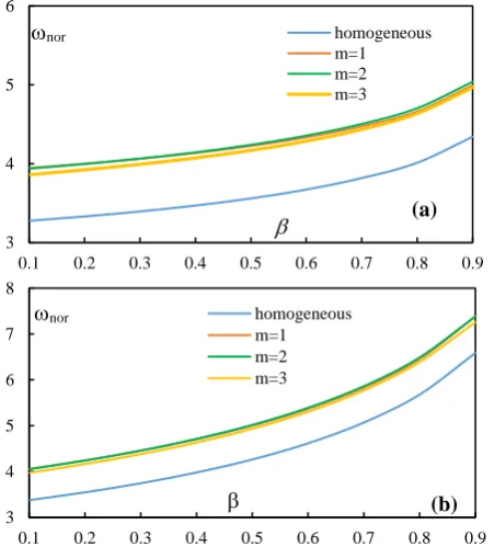
Fig. 2: Variations of the dimensionless fundamental natural frequency of cantilever AFG non-prismatic Timoshenko beam with respect to taper ratio: (a) Case A: cubic variation of moment

of inertia, (b) Case B: quartic variation of moment of inertia

Fig. 3: Variations of the dimensionless fundamental natural frequency of simply supported AFG non-prismatic Timoshenko

beam with respect to taper ratio: (a) Case A: cubic variation of moment of inertia, (b) Case B: quartic variation of moment of

inertia

3 4 5 6

0.1 0.2 0.3 0.4 0.5 0.6 0.7 0.8 0.9 homogeneous m=1 m=2 m=3

3 4 5 6 7 8

0.1 0.2 0.3 0.4 0.5 0.6 0.7 0.8 0.9 homogeneous

m=1 m=2 m=3

3 4 5 6 7 8 9

0.1 0.2 0.3 0.4 0.5 0.6 0.7 0.8 0.9 homogeneous m=1 m=2 m=3

2 3 4 5 6 7 8 9

0.1 0.2 0.3 0.4 0.5 0.6 0.7 0.8 0.9 homogeneous m=1 m=2 m=3

nor

nor



 (a)

(b)

nor nor





(b) (a)

7

Table 1: Convergence of the proposed numerical technique in determination of the first two non-dimensional transverse frequencies (

nor

 ) for axially homogeneous and non-homogeneous Timoshenko beam with two different end conditions

Case Boundary Conditions

Taper ratio

()

Material Mode

Number of terms of power series (n)

Reference

10 20 30 40 50 60

A

Fixed-Free

0.2

Homogenous 1 3.3241 3.3307 3.3307 3.3307 3.3307 3.3307 3.3770[12] 2 13.7643 14.2892 14.2892 14.2892 14.2892 14.2892 14.6120[12]

m=2 1 4.2462 4.0084 3.9963 3.9955 3.9955 3.9954 3.9956[25]

2 15.2479 15.0981 15.0315 15.0216 15.0203 15.0201 15.0247[25]

0.5

Homogenous 1 3.3681 3.5583 3.5591 3.5591 3.5591 3.5591 3.6890[12] 2 26.4336 13.7683 13.7753 13.7754 13.7754 13.7754 14.1280[12]

m=2 1 4.2720 4.2425 4.2390 4.2386 4.2386 4.2385 4.2393[25]

2 14.1372 14.4309 14.4247 14.4223 14.4219 14.4219 14.4282[25]

Hinged-Hinged

0.2

Homogenous 1 7.7001 7.7160 7.7160 7.7160 7.7160 7.7160 7.7370[12] 2 21.1779 24.0858 24.0868 24.0868 24.0868 24.0868 24.1340[12]

m=2 1 7.4702 7.3094 7.2923 7.2904 7.2901 7.2901 7.2921[25]

2 21.8149 23.1395 23.1146 23.1117 23.1113 23.1113 24.1380[25]

0.5

Homogenous 1 6.4839 6.4445 6.4442 6.4442 6.4442 6.4442 6.4740[12] 2 27.0793 21.5906 21.5893 21.5893 21.5893 21.5893 21.6730[12]

m=2 1 6.3442 6.0236 5.9891 5.9850 5.9845 5.9845 5.9897[25]

2 22.6616 20.8746 20.8202 20.8134 20.8126 20.8125 20.8350[25]

B

Fixed-Free

0.2

Homogenous 1 3.5381 3.5462 3.5462 3.5462 3.5462 3.5462 3.6044[12] 2 14.7427 14.6074 14.6074 14.6074 14.6074 14.6074 14.9245[12]

m=2 1 4.4366 4.2498 4.2390 4.2382 4.2381 4.2381 4.2384[25]

2 15.8573 15.4062 15.3488 15.3404 15.3393 15.3392 15.3441[25]

0.5

Homogenous 1 4.0502 4.2609 4.2628 4.2628 4.2628 4.2628 4.3700[12] 2 13.6635 14.6610 14.6736 14.6736 14.6736 14.6736 14.9510[12]

m=2 1 5.0492 5.0201 5.0170 5.0164 5.0164 5.0164 5.0178[25]

2 14.9397 15.3362 15.3412 15.3403 15.3401 15.3401 15.3573[25]

Hinged-Hinged

0.2 Homogenous

1 7.6787 7.6887 7.6887 7.6887 7.6887 7.6887 7.7090[12] 2 22.0085 24.0908 24.0913 24.0913 24.0913 24.0913 24.1380[12]

m=2 1 7.4139 7.2427 7.2246 7.2225 7.2223 7.2222 7.2245[25]

2 22.2912 23.1456 23.1192 23.1160 23.1157 23.1156 23.1398[25]

0.5

Homogenous 1 6.3512 6.2518 6.2508 6.2508 6.2508 6.2508 6.2760[12] 2 31.1362 21.6495 21.6462 21.6462 21.6462 21.6462 21.7210[12]

m=2 1 6.1597 5.7570 5.7128 5.7076 5.7070 5.7069 5.7118[25]

2 22.4540 20.9708 20.9022 20.8936 20.8925 20.8924 20.9191[25]

Table 2: First two normalized natural frequencies (_nor) of homogeneous non-prismatic Timoshenko beam for various tapering ratios and three different end conditions

End Conditions 

Case A Case B

PSM ABAQUS PSM ABAQUS

1

nor



2

nor



1

nor



2

nor



1

nor



2

nor



1

nor



2

nor



Fixed-Free

0.1 3.2756 14.3931 3.4270 14.7040 3.3758 14.5485 3.5280 14.8630

0.2 3.3307 14.2892 3.3770 14.6120 3.5462 14.6074 3.6044 14.9245

0.3 3.3941 14.1540 3.4331 14.5706 3.7444 14.6459 3.8890 14.9890

0.4 3.4689 13.9841 3.6050 14.3280 3.9789 14.6661 4.1760 15.1710

0.5 3.5591 13.7753 3.6890 14.1280 4.2628 14.6736 4.3700 14.9510

0.6 3.6716 13.5235 3.7970 13.8850 4.6159 14.6799 4.7220 14.9620

0.7 3.8170 13.2163 3.9400 13.5970 5.0690 14.6988 5.1770 14.9990

0.8 4.0115 12.8090 4.1420 13.2750 5.6787 14.7883 5.7960 15.1470

0.9 4.3414 12.5482 4.4580 12.9770 6.5879 15.5197 6.6870 15.6730

Hinged-Hinged

0.1 8.0662 24.7480 8.0580 24.7890 8.0596 24.7489 8.0790 24.7890

0.2 7.7160 24.0868 7.7370 24.1340 7.6887 24.0913 7.7090 24.1380

0.3 7.3328 23.3509 7.3560 23.4080 7.2691 23.3638 7.2910 23.4180

0.4 6.9114 22.5253 6.9380 22.5930 6.7933 22.5541 6.8360 22.6690

0.5 6.4442 21.5893 6.4740 21.6730 6.2508 21.6462 6.2760 21.7210

0.6 5.9199 20.5130 5.9550 20.6180 5.6260 20.6185 5.6510 20.7050

0.7 5.3221 19.2531 5.3900 19.4870 4.8997 19.4504 4.9120 19.5340

0.8 4.6449 17.7894 4.6530 17.8940 4.0822 18.2193 4.0010 18.1420

0.9 3.9471 16.3529 3.7270 15.9500 3.2331 17.2697 2.7230 16.3300

0.1 13.5478 28.1785 13.5610 28.1940 13.5499 28.1804 13.5630 28.1960

Numerical Methods in Civil Engineering, Vol. 2, No. 1, September. 2017

Fixed-Fixed

0.2 13.2223 27.7782 13.2380 27.7980 13.2316 27.7869 13.2470 27.8060

0.3 12.8504 27.3007 12.8680 27.3260 12.8739 27.3230 12.8910 27.8001

0.4 12.4222 26.7233 12.4440 26.7550 12.4692 26.7693 12.4890 26.7990

0.5 11.9235 26.0140 11.9500 26.0560 12.0077 26.0987 12.0450 26.1580

0.6 11.3342 25.1249 11.3680 25.1820 11.4759 25.2723 11.5040 25.3210

0.7 10.6238 23.9827 10.6680 24.0620 10.8590 24.2373 10.8880 24.2940

0.8 9.7640 22.4956 9.9230 22.8030 10.1857 22.9803 10.1540 22.9560

0.9 8.8493 20.7515 8.6600 20.4500 9.6445 21.7649 9.2430 21.1020

Table 3: First four non-dimensional transverse frequencies of an axially FG tapered Timoshenko beam (Case A; m=2)

End Conditions 

PSM Shahba et al., 2011 [25]

1

nor



2

nor





nor₃



nor₄



nor1



nor2



nor3



nor4

Fixed-Free

0.1 3.9367 15.1691 31.2133 47.5831 3.9359 15.1577 31.2638 47.7164

0.2 3.9963 15.0315 30.7644 47.2999 3.9956 15.0247 30.8092 47.4362

0.3 4.0645 14.8647 30.2438 46.8099 4.064 14.8611 30.286 46.9481

0.4 4.1441 14.6642 29.6395 46.1213 4.1438 14.6636 29.6818 462610

0.5 4.2390 14.4247 28.9325 45.2184 4.2393 14.4282 28.9791 45.3634

0.6 4.3557 14.1390 28.0895 44.0516 4.3571 14.1513 28.1532 44.2201

0.7 4.5037 13.7902 27.0347 42.4940 4.5090 13.8314 27.1684 42.763

0.8 4.7033 13.3594 25.5978 40.1103 4.7180 13.4793 25.9735 40.8666

0.9 5.0387 13.1333 24.2837 37.5732 5.0371 13.1700 24.5212 38.2968

Hinged-Hinged

0.1 7.6547 23.7153 41.7046 57.7388 7.6545 23.7369 41.821 57.8739

0.2 7.2923 23.1146 41.0094 59.1739 7.2921 23.1346 41.1203 59.4848

0.3 6.8978 22.4418 40.2002 58.4650 6.8965 22.4604 40.3053 58.7642

0.4 6.4659 21.6832 39.2519 57.4616 6.4653 21.7002 39.3507 57.7558

0.5 5.9891 20.8202 38.1274 56.2303 5.9879 20.8350 38.2191 56.5105

0.6 5.4572 19.8273 36.7724 54.6960 5.454 19.8372 36.8536 54.9547

0.7 4.8588 18.6746 35.1070 52.7350 4.8448 18.6634 35.1618 52.9529

0.8 4.1974 17.3737 33.0537 50.1271 4.1244 17.2364 32.975 50.2463

0.9 3.5183 16.1334 30.9399 47.1922 3.2016 15.3775 29.9011 46.2153

Fixed-Fixed

0.1 12.4651 26.3822 42.9600 59.3072 12.4689 26.4153 43.0904 59.6829

0.2 12.2086 26.0701 42.4941 59.1799 12.2126 26.1023 42.6211 59.4873

0.3 11.9130 25.6923 41.9527 58.7677 11.9172 25.7236 42.0759 59.0576

0.4 11.5697 25.2288 41.3095 58.1325 11.5739 25.2590 41.4283 58.4306

0.5 11.1664 24.6511 40.5240 57.2971 11.1706 24.6797 40.6374 57.5925

0.6 10.6865 23.9170 39.5325 56.1983 10.6896 23.9424 39.6375 56.4814

0.7 10.1080 22.9657 38.2334 54.7086 10.1036 22.9773 38.3161 54.9627

0.8 9.4236 21.7335 36.4770 52.6149 9.3634 21.6575 36.4588 52.7499

0.9 8.7203 20.3117 34.2502 49.6266 8.3590 19.6945 33.5615 49.1234

After noticing the results tabulated in Table 1, it can be stated that for a satisfactory result, especially at higher modes, the minimum number of terms for the power series (n) must be 30. In the case of taper ratios higher than 0.8, it is worthy to note that 50 terms of power series must be taken into account to calculate the values of free transverse frequencies with an acceptable error rate.

In what follows, the precision of the proposed numerical approach is verified by applying to homogenous non-prismatic beams (Cases A & B). The first two natural frequencies for various types of boundary conditions and different values of taper ratios () are tabulated in Table 2. It can be recognized that the results are in an excellent agreement with those acquired by ABAQUS software. In the case of fixed-fixed and hinged-hinged, it is also obvious that the natural frequency decreases with an increase in taper ratio, which has resulted from the reduction in cross-sectional area and moment of inertia and consequently mass and stiffness of the elastic member. In order to evaluate the

values of dimensionless natural frequency parameters with an acceptable error rate, 30 terms of power series have been taken into account.

The dimensionless natural frequencies (_nor) relating to the first four vibrational modes of AFG non-prismatic beam for a non-homogeneity index of m=2 have been arranged in Tables 3-4. Table 3 consists of the results of case A, while Table 4 summarizes the results of case B. The obtained results by the proposed numerical technique have been compared with those reported in [25].

After reviewing the results presented in Tables 2 to 4, it can be stated that the current procedure based on power series expansions is applicable for the higher vibration modes, as well as for the first one with excellent accuracy. Subsequently, the influences of tapering parameter () on dimensionless natural frequencies of FG non-prismatic beam by considering the non-homogeneity index m=1, 2 and 3 for fixed-free, simply supported and fixed-fixed are respectively illustrated in Figs. 2 to 4.

9

Table 4: First four non-dimensional transverse frequencies of an axially FG Timoshenko beam (Case B; m=2)

End Conditions 

PSM Shahba et al., 2011 [25]

1

nor



2

nor



3

nor



4

nor



1

nor



2

nor



3

nor



4

nor



Fixed-Free

0.1 4.0500 15.3227 31.3305 47.6892 4.0492 15.3129 31.3795 47.8232

0.2 4.2390 15.3488 31.0109 47.5171 4.2384 15.3441 31.0546 47.655

0.3 4.4569 15.3591 30.6379 47.1495 4.4565 15.3579 30.6798 47.2907

0.4 4.7121 15.3550 30.2060 46.6035 4.7121 15.3573 30.2496 46.7483

0.5 5.0170 15.3412 29.7063 45.8744 5.0178 15.3487 29.7571 46.0287

0.6 5.3904 15.3272 29.1206 44.9278 5.3931 15.3467 29.1962 45.1172

0.7 5.8617 15.3291 28.3980 43.6495 5.8695 15.3856 28.568 43.9835

0.8 6.4890 15.4500 27.5444 41.7703 6.5009 15.5568 27.9102 42.5941

0.9 7.3877 16.2212 27.5672 40.9326 7.3787 16.1537 27.4806 41.0442

Hinged-Hinged

0.1 7.6269 23.7152 41.7024 57.7920 7.6269 23.7369 41.8193 57.9246

0.2 7.2246 23.1192 41.0122 59.2204 7.2245 23.1398 41.1243 59.5225

0.3 6.7765 22.4586 40.2175 58.4758 6.7764 22.4783 40.3248 58.7787

0.4 6.2757 21.7236 39.2970 57.4878 6.2755 21.7423 39.3994 57.7881

0.5 5.7128 20.9022 38.2207 56.2962 5.7118 20.9191 38.3174 56.5841

0.6 5.0758 19.9820 36.9481 54.8345 5.0709 19.9917 37.0337 55.1026

0.7 4.3556 18.9660 35.4340 53.0095 4.3295 18.9367 35.4785 53.2304

0.8 3.5706 17.9552 33.7316 50.7399 3.4452 17.7204 33.5322 50.7616

0.9 2.7630 17.2371 32.3439 48.6833 2.3193 16.2962 30.9578 47.2473

Fixed-Fixed

0.1 12.4772 26.4043 42.9790 59.3417 12.4812 26.4376 43.1098 59.7067

0.2 12.2385 26.1194 42.5353 59.2401 12.2429 26.1524 42.6634 59.5335

0.3 11.9689 25.7762 42.0208 58.8343 11.9737 25.8089 42.1461 59.1273

0.4 11.6631 25.3581 41.4118 58.2223 11.6683 25.3905 41.5341 58.5279

0.5 11.3145 24.8425 40.6731 57.4215 11.3199 24.8744 40.7919 57.7257

0.6 10.9163 24.1982 39.7513 56.3718 10.92 24.227 39.8636 56.6668

0.7 10.4689 23.3896 38.5698 54.9693 10.4579 23.3976 38.657 55.2354

0.8 10.0208 22.4278 37.0543 53.0603 9.9207 22.301 37.005 53.1931

0.9 9.7257 21.5393 35.4151 50.5748 9.301 20.7781 34.554 49.9856

Fig. 4: Variations of the dimensionless fundamental natural frequency of fixed-fixed AFG non-prismatic Timoshenko beam with respect to taper ratio: (a) Case A: cubic variation of moment

of inertia, (b) Case B: quartic variation of moment of inertia

Regarding Eq. (20), it is obvious that by increasing the gradient index (m) from 1 to 3, the volume fraction of Zirconia is increased and as a result, a stiffer and also heavier beam is acquired. Besides, as taper ratio is increased from 0.1 to 0.9, the moment of inertia and cross-sectional area are reduced and accordingly both stiffness and mass of beam are gradually diminished. Therefore, the beam easily becomes weaker and lighter. Since the free transverse vibration in the absence of damping is dependent on both the mentioned terms (mass and stiffness), it is not possible to predict the variations of natural frequency with respect to non-homogeneity index (m) and tapering parameter () concurrently. This fact can be easily observed in Figs. 2-4. 3.2. Example 2- Axially functionally graded tapered Timoshenko beam under axial load

Natural frequencies and vibrational mode shapes of structural members subjected to a compressive or tensile concentrated axial load are key factors in the design of different structures ranging from civil engineering to mechanical constituents. Therefore, exact calculation of bending vibration characteristics of flexural members could considerably help design engineers to improve the quality and the performance of structures. To study the effect of axial load on free vibration behavior of Timoshenko beam, another example is presented. In this regard, an elastic beam with rectangle cross-section whose height tapers linearly along the member axis is taken into account. Therefore, the cross-sectional area and moment of inertia are identical to Case A of the first example. 8

9 10 11 12 13 14

0.1 0.2 0.3 0.4 0.5 0.6 0.7 0.8 0.9 homogeneous m=1 m=2 m=3

8 9 10 11 12 13 14

0.1 0.2 0.3 0.4 0.5 0.6 0.7 0.8 0.9 homogeneous m=1 m=2 m=3

nor

nor





(b) (a)

Numerical Methods in Civil Engineering, Vol. 2, No. 1, September. 2017

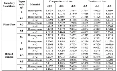
Table 5: First non-dimensional vibration frequency (_nor) for Timoshenko beam subjected to a concentrated axial load at its ends

Boundary Conditions

Taper ratio

()

Material

Compressive axial load Tensile axial load

+0.2 +0.5 +0.8 -0.2 -0.5 -0.8

Fixed-Free

0 Homogenous 3.1457 2.6045 1.8544 3.7094 4.0605 4.3699 m=2 3.7542 3.1076 2.1540 4.4016 4.7945 5.1359

0.1 Homogenous 3.1240 2.5695 1.7841 3.7516 4.1026 4.4114 m=2 3.7992 3.1489 2.1788 4.4452 4.8353 5.1733

0.3 Homogenous 3.2884 2.7339 1.9488 3.8565 4.2059 4.5116 m=2 3.9142 3.2612 2.2589 4.5505 4.9301 5.2560

0.5 Homogenous 3.4433 2.8879 2.0874 4.0034 4.3442 4.6404 m=2 4.0853 3.4448 2.4222 4.6932 5.0501 5.3549

0.7 Homogenous 3.7128 3.1899 2.4232 4.2312 4.5430 4.8124 m=2 4.3774 3.8005 2.8264 4.9066 5.2121 5.4714

Hinged-Hinged

0 Homogenous 7.5362 5.9698 3.8042 9.2186 10.3010 11.2794 m=2 7.1964 5.7341 3.7004 8.7594 9.7620 10.6669

0.1 Homogenous 7.2550 5.7575 3.6930 8.8663 9.9032 10.8408 m=2 6.9012 5.5056 3.5600 8.3901 9.344 10.2043

0.3 Homogenous 6.6120 5.2591 3.3947 8.0655 9.0003 9.8452 m=2 6.2339 4.9913 3.2492 7.5528 8.3946 9.1521

0.5 Homogenous 5.8396 4.6698 3.0566 7.0923 7.8959 8.6208 m=2 5.4311 4.3725 2.8759 6.5458 7.2528 7.8864

0.7 Homogenous 4.8697 3.9404 2.6586 5.8587 6.4891 7.0441 m=2 4.4146 3.5852 2.3977 5.2762 5.8167 6.2975

The natural frequencies are also carried out for two cases: axially non-homogeneous and homogeneous beams. In the case of axially FG member, the distribution of modulus of elasticity and density of material are contemplated to vary in the longitudinal direction with a power-law formulation as expressed in Eq. (20). In this case, the material non-homogeneity parameter (m) is assumed to be equal to 2. Moreover, the vibration frequency is acquired for five different tapering parameters: 0, 0.1, 0.3, 0.5 and 0.7. The following non-dimensional quantity corresponding to point external axial force is also used:

cr

P P

 (21)

Non-dimensional critical loads (Pcr) of the contemplated members made of homogenous material are obtained using ABAQUS software and those related to axially functionally graded beams are stated in Shaba et al., 2011 [25]. In the case of compressive axial force,  is negative, however; this parameter is positive for a tensile load. The vibration frequencies are obtained for 0.2, 0.5, 0.8  . It is noteworthy that non-dimensional free vibration frequencies are computed for homogenous and AFG beams with simply supported and clamped-free boundary conditions. Results are tabulated in Table 5.

In case of tensile axial load, fundamental frequency is observed to increase with an increase in . This is due to the fact that the free transverse vibration in the absence of damping and harmonic external loads is directly proportional to stiffness. In general, the effect of a tensile axial load is to decrease the deflection and increase stiffness of the member and consequently the natural frequencies, as can be seen from the results presented in Table 5. While in case of compressive axial force beam, natural frequency is observed to decrease with an increase in normalized axial force parameter ().As compressive axial force approaches

the critical buckling load, the transverse deflection of the member increases noticeably and as a result, the stiffness of the member vanishes and a weaker member is obtained. Therefore, a significant decrease in vibration frequency of the member is observed (see Table 5).

3.3. Example 3- Non-prismatic Timoshenko beam with exponential distribution of material properties

In this example, free vibration analysis is accomplished for an AFG double-tapered Timoshenko beam whose

cross-sectional area and moment of inertia vary over the member’s

length according to Case C (Eq. (19c)). For such a member, it is also assumed that the material properties including Young’s modulus of elasticity and the mass density change exponentially along the beam as:

0 5 0

( ) .

E  E e  (22a) 0 5

0

( ) e. 

    (22b) FGM possesses properties that vary exponentially through longitudinal direction is one of the most special cases of composite material that few numerical methods are able to solve its governing differential equation. Based on the power series method, all variable terms in motion equations are presented in a polynomial form. In the presence of exponential variations, the Maclaurin series expansion should be adopted. The explicit forms of Maclaurin series for material properties (Eq. (22)) are thus defined as:

0 0

( 0.5) ( )

!

i i i

E E

i 









  (23a)

0 0

( 0.5) ( )

!

i i i i











    (23b) The first two non-dimensional free frequency parameters for different combinations of height and width tapering ratios ( and ) with two types of end conditions are tabulated in Table 6.

11

Table 6: First two dimensionless natural frequencies (_nor) for exponential FGM double tapered Timoshenko beam with two different

end conditions

End conditions

Height taper ratio ()

Width taper ratio ()

0.0 0.2 0.4 0.6 0.8

1

nor





nor₂



nor1



nor2



nor1



nor2



nor1



nor2



nor1



nor2

Hinged-Hinged

0.0 7.987 24.252 7.930 24.242 7.831 24.213 7.652 24.133 7.273 23.861

0.2 7.290 23.111 7.222 23.116 7.115 23.110 6.934 23.073 6.572 22.898

0.4 6.463 21.678 6.386 21.698 6.272 21.717 6.089 21.726 5.746 21.653

0.6 5.450 19.814 5.366 19.853 5.247 19.902 5.064 19.962 4.741 20.003

0.8 4.119 17.211 4.033 17.277 3.914 17.367 3.737 17.497 3.441 17.692

Cantilever

0.0 3.883 15.259 4.124 15.596 4.444 16.027 4.898 16.629 5.614 17.638

0.2 3.995 15.020 4.238 15.339 4.560 15.750 5.017 16.329 5.740 17.316

0.4 4.143 14.658 4.387 14.960 4.711 15.351 5.171 15.908 5.902 16.875

0.6 4.356 14.143 4.601 14.428 4.927 14.799 5.391 15.335 6.128 16.284

0.8 4.715 13.457 4.962 13.723 5.291 14.075 5.756 14.589 6.494 15.520

Table 7: The first three normalized natural frequencies of clamped-free Timoshenko beam and Euler-Bernoulli beam

 Timoshenko Beam Theory Euler-Bernoulli Beam Theory L/b0

1 nor



2 nor



3 nor



1 nor



2 nor



3 nor



0.2

5 3.7420 18.0348 41.9204

3.8551

3.8551

21.0571

21.0568

56.6379[3]

56.6303[6]

10 3.8257 20.1527 51.3881

50 3.8539 21.0180 56.3842

100 3.8548 21.0470 56.5684

0.4

5 4.1948 17.622 39.7719

4.3187

4.3187

20.0505

20.0500

51.3423[3]

51.3346[6]

10 4.2866 19.3428 47.4121

50 4.3174 20.0200 51.1542

100 4.3184 20.0424 51.2895

0.5

5 4.4931 17.3940 38.5312

4.6251

4.6252

19.5482

19.5476

48.5870[3]

48.5789[6]

10 4.5909 18.9289 45.2611

50 4.6237 19.5214 48.4274

100 4.6247 19.5407 48.5317

It is concluded again that the geometrical parameter is an important parameter in determining the lower-order normalized natural frequencies for simply supported and cantilever exponential FG Timoshenko beams.

3.4. Example 4- Tapered Timoshenko beam versus tapered Euler-Bernoulli beam

To depict the difference between the free vibration frequencies of Euler-Bernoulli beam theory and those of Timoshenko beam model, this illustrative example is also considered. In the case of double tapered beam, both the height and width of the beam cross-section decrease linearly along the member’s axis with the same tapering ratio (), as expressed in Eq. (19b). For different values of L/b0, the first

three natural frequencies are calculated for fixed-free beams and the results are arranged in Table 7. The values of taper parameter (and the type of boundary conditions are selected in such a way that make comparison possible with other available references in the case of non-prismatic Euler-Bernoulli beam (Banerjee et al., 2006 [6]; Attarnejad, 2010 [3]). From Table 7, one can see that the natural frequencies calculated by employing Euler-Bernoulli theory (EBT) are

overestimated. The difference between EBT and shear deformation theory (Timoshenko beam model) is small for slender beams (L/b0>50). Note that for deep members

(L/b0<10), this difference is significant especially at higher

modes (see Table 7). This is owing to the fact that the influences of shear deformation and rotatory inertia are ignorable in the Euler-Bernoulli theory. In general, the effects of both mentioned parameters are to increase the deflection and reduce the stiffness, as well as natural frequencies.

4. Conclusions

In the present study, the free transverse vibration analysis of elastic non-prismatic Timoshenko beam made of axially functionally graded material (AFGM) with arbitrary boundary conditions has been investigated using a numerical approach. The effect of point axial load which is tangential to the longitudinal axis of beam on bending vibration frequency is also taken into consideration.

In presence of arbitrary variation in geometrical and material properties, the governing motion equations of Timoshenko beam include a pair of second-order differential equations with variable coefficients. Therefore, the vibration analysis