Spatial Variations of
β
-Convergence Coefficient in
Asia (The GWR Approach)
Shekoofeh Farahmand Majid Sameti Seyed Salahaldin Sasan
Received: 2013/03/11 Accepted: 2013/12/11
Abstract
he economic convergence concept arises from the Solow-Swan growth model. Accordingly, two hypotheses are considered: absolute and conditional convergence. The first implies the convergence of economies towards a steady-state. The second hypothesis is based on the convergence of each economy toward its own steady-state. Indeed, it refers to different structures of economies. In experimental studies, for testing the conditional hypothesis, different determinants are entered in the growth model to capture the differences in structures. However,
one coefficient is estimated for β-convergence and one convergence
speed is obtained. This paper examines the convergence hypotheses for Asian countries over the period of 1999-2009 using the geographically weighted regression (GWR) approach. GWR provides useful means for dealing with spatial variation in convergence speed. In this way, convergence coefficients can be computed for considered countries. The results show that, speed of convergence varies over different countries. Also, the spatial variation of steady- state incomes is significant.
Keywords: Solow-Swan Growth Model, β-Convergence, Spatial
Variations, GWR.
Assistant Professor, Economic Department, University of Isfahan.
Associate Professor, Economic Department, University of Isfahan.
1- Introduction
The study of the convergence process on the regional and international levels has been one of the main subjects of regional science and macroeconomic literature for decades. As stated by Abramovitz (1986), convergence implies a long run tendency towards the equalization of income per capita or product levels.
In fact, convergence hypothesis tries to answer two main questions. First, do the dispersions of per capita incomes of countries (regions) decrease over time? This type of convergence is called σ-convergence. Second question is whether “poor” countries, as measured by low per capita incomes, display faster growth rates in per capita income than “rich” countries with higher per capita incomes. The second type is named β-convergence in the growth literature (Durlauf, Johnson and Temple, 2005).
An important contribution by Baumol (1986) has stimulated a large number of studies examining the convergence hypothesis at the international level. Rey and Montouri (1999) have believed that since these studies have been informed by different theoretical perspectives (i.e., neo-classical models versus endogenous growth models) and have employed different empirical strategies (i.e., cross-sectional versus time-series versus panel data), the existing empirical evidence on convergence between nations is subject to much debate. The results of empirical research on the subject has not yet reached a common answer as to whether, and under which conditions, convergence actually takes place (Debarsy and Eture, 2007).
techniques to consider space. Taking space into account in the econometric regression has two dimensions: spatial dependence and spatial heterogeneity. This study reconsiders the question of economic income convergence for Asian countries through spatial econometrics by considering both spatial dependence and spatial heterogeneity. The main contribution of the study is that in addition to the estimated global parameters of the convergence model, local parameter estimates are also obtained, taking into account the heterogeneity associated with the cross-sectional data analysis. Indeed, the main idea in the conditional β-convergence is that each economy converges toward its own steady-state. For defining different steady-state levels of incomes, in addition to the initial income level, other variables than have been entered in the growth model (Barro and Sala-i-Martin, 1995), but only one speed of convergence is obtained by estimating the specified model. In this paper, we obtain the convergence speed of each country through GWR approach (some studies, e.g. Durlauf and Johnson (1995), Hansen (1996), and Arbia and Basile (2005), have estimated different steady-state levels and convergence coefficients for groups of countries by multiple regimes).
The layout of the paper is as the following. In Section 2, we present a review of β-convergence concept. Regression specifications of the convergence model by considering spatial dependence and spatial heterogeneity are presented in section 3. Section 4 reports the results of an empirical analysis based on the 43 Asian countries data in the period of 1999-2009. The paper closes with a summary in section 5.
2- Convergence Concepts
coefficient of variation (Bernard and Jones, 1996) of the log of per capita income. This form of convergence has been referred to as σ-convergence. A second form of convergence, named β-convergence, which has primarily been the focus of macroeconomists, occurs when poor regions grow faster than rich regions, resulting in the former eventually catching up to the latter in per capita income levels (Rey and Montouri, 1999).1
The traditional neoclassical model of growth, originally set out by Solow (1956) and Swan (1956), and, following the work of Ramsey (1928), subsequently refined by Cass (1965) and Koopmans (1965), has provided the theoretical background for the empirical analyses on β-convergence (Magrini, 2004). This model is extracted from a production function, assuming a closed economic system, exogenous saving rates and a production function based on decreasing productivity of capital and constant returns to scale. The model shows that the growth rate experienced by the economy is negatively related to the initial level: the lower the initial level, the further the economy is from its balanced growth path, and the higher its growth rate.
Barro and Sala-i-Martin (1992) suggested the following cross-sectional statistical model, in matrix form:
= − 1 − + ℎ ~ . . (0, ) (1)
y0 and yT are the GDP per capita in logarithms in current and initial years, respectively. ϵ is the error term. β is the speed of adjustment to the steady-state, i.e. the rate at which the economies approach their steady-state growth paths.
Convergence is observed if β is positive and significant. The equation (1) shows that the growth rate is negatively correlated with the initial level of GDP per capita. This is absolute (unconditional) β-convergence because the long-run equilibrium is the same for all economies. Indeed, economies share the same structural characteristics [in terms of human capital, saving rate, production function …] (Debarsy and Ertur, 2007). Therefore, poor economies grow faster than rich ones only if they all share the same steady-state. If structural characteristics differ between economies, each economy tends to its own long-run equilibrium, which is unique and determined by the characteristics of the economy. This is conditional convergence and some other variables are entered to the model holding constant the steady-state equilibrium of each economy.
3- Methodology
Some studies have tried to considered direct variables for interregional flows in the growth model. For example, Barro and Sala-i-Martin (1995) have tested the role of migration flows on convergence. However, such a direct approach is limited because the lack of needed data.
An alternative and indirect way to control for the effects of interregional flows (or spatial interaction effects) on growth and convergence is through spatial dependence models and spatial econometric techniques. As emphasized by Rey and Montuori (1999), the literature on spatial econometrics offers a rich set of procedures for testing for the presence of spatial effects (Anselin, 1988; Anselin & Bera, 1998; Anselin & Florax, 1998; and Anselin and Rey, 1991). Moreover, within the cross sectional regression approach, there exist a number of estimators for models that treat spatial effects explicitly (Magrini, 2004).
It has been defined two spatial effects in the spatial econometrics literature: spatial dependence (autocorrelation) and spatial heterogeneity. There are two ways to take spatial dependence into account. The first is through re-specifying a model as a Spatial Auto-Regressive (SAR) model in which the spatial lag of the dependent variable is entered in the set of explanatory variables. If w is a row-standardized matrix of spatial weights describing the structure and intensity of spatial effects, based on equation (1), the SAR model would be:
= − 1 − + + (2)
its neighbors. w is defined according to the contiguity, so that wij take values of 0 or 1 accordance to the absence or presence of a contiguity relationship between countries i and j. Ordinary least squares (OLS) to the SAR model are inconsistent and alternative estimators based on maximum likelihood (ML) and instrumental variables should be employed (Anselin, 1988). In the paper, ML estimators are considered.
An alternative way to incorporate the spatial effects is via the spatial error model or SEM (Anselin and Bera, 1998; Arbia, 2006). This leaves unchanged the systematic component and models the error term in equation (1) as an autoregressive random field. That is:
= − 1 − + (3)
= . . +
different convergence speeds toward steady-state income. Meanwhile, different steady-state income levels are expected. Thus, it would be unrealistic to consider a global β for all countries. Different β coefficients can be calculated by the technique of geographically weighted regression (GWR) which is introduced by Brudson, Fotheringham, and Charlton (1996). GWR considers spatial non-stationarity in relations. One advantage of this technique is that it corporates local spatial relations into the regression framework in an intuitive and explicit manner (Fotheringham, Brudson & Charlton, 2002).
Using GWR in estimating our model allows capturing spatial variations in β -convergence coefficient. In each country’s individual regression, other countries in the sample are weighted by their spatial proximity. In GWR approach, the model can be rewritten as:
= ( , ) − 1 − ( , ) + (4)
where (ui, vi) denotes the coordinates of the ith point in space. This model would show that spatial variations in steady-state and β coefficient might exist and GWR provides a way through which these variations can be measured.1
However, there are more unknown parameters than degrees of freedom in this GWR model. Hence, the local parameters are obtained using regression. “In GWR, observations are weighted in accordance to their proximity to location i so that the weighting of an observation is no longer constant in calibration and varies with i. Therefore, data from observations close to i are
weighted more that data from observations farther away” (Fotheringham, Brudson & Charlton, 2002, p. 53). Then,
( , ) =
( ( , ) ) ( , ) (5)
β denotes the estimate of β1, and W(u , v ) is an n by n spatial weight matrix whose off-diagonal elements are zero and whose diagonal elements represent the geographical weighting of each of the n observed data foe regression point i. The estimator in equation (5) is a weighted least squares estimator but rather than having a constant weight matrix, the weights in GWR vary according to the location of point i. Hence, the weight matrix has to be computed for each point i and the weights depict the proximity of each data point to the location of i with points in closer proximity carrying more weight in the estimation of the parameters for location i (Fotheringham, Brudson & Charlton, 2002).
In estimating the parameters in a GWR equation, it is important to choose a criteria to define the weighting matrix. Brudson, Fotheringham, and Charlton (1996, 1997) specify Wij as a continuous and decreasing function based on distance between pairs of observations. Different functions are used for specifying Wij (Brudson, Fotheringham & Charlton, 1996, 1997). In Wij, the weights are allowed to decay with distance following a Gaussian decay function for a fixed kernel. However, the kernels should be allowed to vary spatially. This is done by different methods. One way is based on the N nearest neighboring weighting with a bi-square decay function (for a more detailed explanation of defining the spatial weights matrix for fixed and adaptive kernels see Fotheringham, Brudson, & Charlton, 2002). In this
study, the optimal number of neighboring unites is determined through an iterative process to minimize the Akaike information criteria (AIC).
The local regression model for this study was calibrated using GWR software developed by Fotheringham, Brunsdon & Charlton (2003). The software provides t-statistics for each parameter at each data point and R2 values.
An approximate likelihood ratio test, based on the F-test, can be used to compare the relative performance of the GWR and OLS models to replicate the observed data (Fotheringham, Brunsdon & Charlton, 2002). This test is based on the result that the distribution of the residual sum of squares of the GWR model divided by the effective number of parameters may be reasonably approximated by a χ distribution with effective degrees of freedom equal to the effective number of parameters. Thus,
= (6)
where RSS1 and RSS2 are the residual sum of squares of the OLS model and GWR model, respectively. d1 and d2 are the degrees of freedom for the OLS and GWR model, respectively.
For testing the significance of spatial variations of estimated parameters, the Mont Carlo test is used which is explained in the Fotheringham, Brunsdon and Charlton (2002) in detail.
The specified models are estimated for 43 Asian countries whose data are available.1 The data are retrieved from the World Bank website for the period of 1999-2009.
4- The Empirical Results
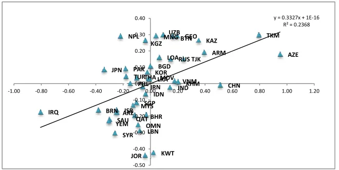
For having an initial view of spatial dependence, before estimating models, we trace the Moran’s I scatter plots for economic growth rates of considered countries, suggested by Anselin (1993). This figure plots the standardized growth rate of a country against its spatial lag (also standardized). A country’s spatial lag is a weighted average of the growth rates of its neighbors, with the weights being obtained from the simple contiguity matrix. Quadrants I and III pertain to positive forms of spatial dependence while the remaining two represent negative spatial dependence (Rey and Montoury, 1999). The trend line in figure 1 verifies the positive spatial dependence for growth rates. As expected, high growth countries (most newly independent states) are located in Quadrant I and most Persian-Gulf countries are in Quadrant III.
Figure 1: Moran Scatter Plot for Growth Rates of Asian Countries, 1999-2009.
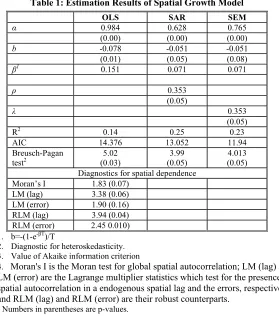
Table 1 reports the estimation results for a cross-sectional regression of the growth model (1) for the 34 considered countries and two spatial
UZB TKM
MNG GEOBTN NPL
KAZ KGZ
ARM AZE
LOARUSTJK BGD PAK
JPN KOR
TURTHA MDVLKA VNMKHM
PHLIRN IND CHN IDN SGP MYS ISR BRN IRQ ARE BHR QAT SAU YEM OMN LBN SYR KWT JOR
y = 0.3327x + 1E-16 R² = 0.2368
-0.50 -0.40 -0.30 -0.20 -0.10 0.00 0.10 0.20 0.30 0.40
dependence models specified in equations (2) and (3). The results in the second column of the table provide support for β-convergence, so that the estimated coefficient of the initial per capita GDP is –0.078 and statistically significant. The implied annual rate of convergence over the study period is reported to be 1.5 % which is very low.
Table 1: Estimation Results of Spatial Growth Model
OLS SAR SEM
α 0.984 0.628 0.765
(0.00) (0.00) (0.00)
b -0.078 -0.051 -0.051
(0.01) (0.05) (0.08)
β1 0.151 0.071 0.071
ρ 0.353
(0.05)
λ 0.353
(0.05)
R2 0.14 0.25 0.23
AIC 14.376 13.052 11.94
Breusch-Pagan
test2 (0.03) 5.02 (0.05) 3.99 (0.05) 4.013
Diagnostics for spatial dependence Moran’s I 1.83 (0.07)
LM (lag) 3.38 (0.06) LM (error) 1.90 (0.16) RLM (lag) 3.94 (0.04)
RLM (error) 2.450.010)
1. b=-(1-e-βT)/T
2. Diagnostic for heteroskedasticity. 3. Value of Akaike information criterion
4. Moran's I is the Moran test for global spatial autocorrelation; LM (lag) and
LM (error) are the Lagrange multiplier statistics which test for the presence of spatial autocorrelation in a endogenous spatial lag and the errors, respectively; and RLM (lag) and RLM (error) are their robust counterparts.
* Numbers in parentheses are p-values.
significant a Moran’s I, the sample is not randomly distributed and spatial autocorrelation is present among observations. However, this test does not specify the nature of dependence (Debarsy and Ertur, 2007).
As seen in table 1, the Moran's I statistic is positive and significant, confirming the presence of positive spatial autocorrelation. Four Lagrange Multiplier (LM) tests have been performed in order to discriminate between two forms of spatial dependence (spatial autocorrelation of an endogenous spatial lag or of the error term). Results of both LM (lag) and RLM (lag) are more significant than their counterpart for the auto-correlated errors model. According to the decision rule elaborated by Anselin and Rey (1991) and modified by Anselin and Florax (1995), it seems that the presence of spatial dependence is better modeled by the endogenous spatial lag than by spatial error autocorrelation (see also Florax, Folmer & Rey, 2003).
Columns 3 and 4 in table 2 represent the estimated results of SAR and SEM models. Their estimated convergence coefficients are smaller than the OLS estimate. Consequently, the speed of β-convergence is very slow (about 0.07% per year). It can be because of the different conditions of considered countries.
In the SAR model, the estimated spatial coefficient, ρ, is positive and statistically significant. As a result, it can be stated that the growth of each country is affected by the growth of its neighbors. In other words, there is some evidence suggesting that having high growth neighbors can be a positive factor for each country. Similar to the SAR model, the SEM model also shows positive and significant contiguity effects on economic growth rates of sample countries. On the whole, these results are common in positive spatial effects with some other studies including Rey and Montoury (1999), and Arbia and Basile (2005).
above works, the cases of studies are the states of the US, and Italian provinces, respectively. For these cases, observations have more similarities. However, the case of this study is Asian countries which have different structures and socio-economic conditions. Hence, it seems that the spatial heterogeneity models should come into consideration. Consequently, we estimate the equation (4) using GWR technique. This technique produces estimates for every point in space by using a subsample of data information from nearby observations. As a result, we will achieve to a unique steady-state income and β-convergence coefficient for each sample country.
Table 2: Tests Based on the Monte Carlo Significance Test
Parameter p-value
Constant 0.01**
Lny0 0.04*
* and ** denote significance at the5% and 1% levels.
According to table 2, it appears that spatial variations are significant for both intercept and β-coefficient. Therefore, it can draw the tentative conclusion that steady-state incomes and convergence speeds would varies spatially. Table 3 presents the descriptive statistics of the parameter estimates from OLS and GWR models.
Table 3: Global and Local Parameter Estimates of the Growth Model
Variables Minimum quartile Lower Median OLS quartile Upper Maximum Constant -0.8263 0.0919 0.634 0.984*** 1.067 2.572
(0.00)
Lny0 -0.289 -0.099 -0.039 -0.078*** 0.020 0.113
(0.01)
0.50 0.14
AIC 20.612 33.436
F statistic 3.572***
Values in parentheses are the p values. *** denotes significance at the 1% level.
Besides, the F statistic, reported at the bottom of Table 3, provides the evidence to suggest that the GWR model significantly improves model fitting over the OLS model.
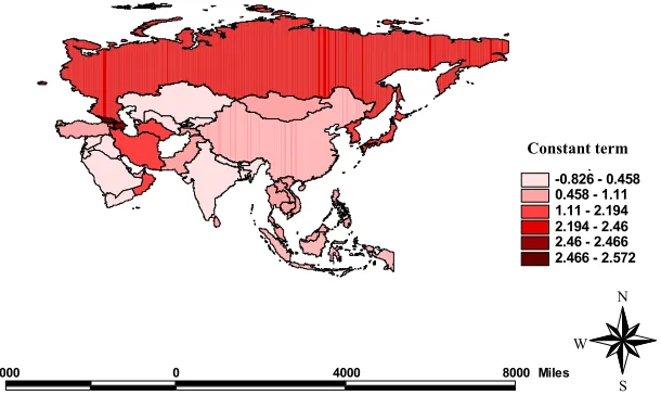
Figure 2 illustrates the spatial distribution of the constant term which would appear the differences of steady-state income levels across considered countries.
Figure 2: Spatial Distribution of the Constant term
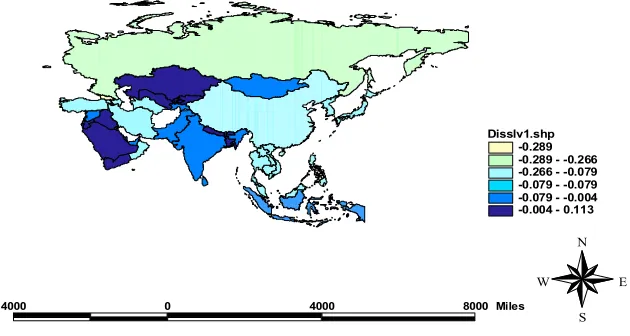
In the same way, figure 3 demonstrates the spatial distribution of convergence coefficients. As it can be seen, the differences in convergence coefficients are basically considerable, which can be due to structural socio-economic differences of countries. According to the estimated coefficients of Lny0, the speed of convergence (β-coefficient) would be in a range of 3.4% (for Georgia) to 0.004% (for India).
The estimated coefficients for initial income per capita of some observations are negative. Nevertheless, none of them are statistically
Disslv1.shp -0.826 - 0.458 0.458 - 1.11 1.11 - 2.194 2.194 - 2.46 2.46 - 2.466 2.466 - 2.572
4000 0 4000 8000 Miles
N
E W
significant except to the Saudi Arabia. In other words, it can imply divergence instead of convergence for the case.
The worthwhile point here is that there is no correlation between the income level and β-convergence coefficient, so that the correlation coefficient is 0.058. It would mean that for the case of the present study, poorer countries may not necessarily have a higher speed of convergence. Common in the constant term, the relatively wide range of the geographically estimated convergence coefficients could presents structural differences of considered countries.
Figure 3: Spatial Distribution of β-Convergence Coefficient
5- Conclusion
In economics literature, there are so many works which have tried to analyze regional growth behavior and test regional convergence within a cross-sectional regression. In the last two decades, some studies have considered spatial dependence in their models through spatial econometric techniques. In particular, the present paper has considered both two aspects
Disslv1.shp -0.289 -0.289 - -0.266 -0.266 - -0.079 -0.079 - -0.079 -0.079 - -0.004 -0.004 - 0.113
4000 0 4000 8000 Miles
N
E W
of spatial effects, namely spatial dependence and spatial heterogeneity in estimating the convergence process among Asian countries. On the one hand, these countries have common borders, and on the other hand they have distinct structures and conditions. Thus, two aspects of spatial effects would be important.
Most present studies have supposed the same economic, social and political conditions for different countries and examined the convergence hypothesis. Some have tried to bring differences into consideration through defining clusters or regimes of countries. One beneficial way here is GWR which yields locally different parameters.
According to the results, the spatial variations of β-convergence coefficient are statistically significant. It would mean that each country can converge or diverge by its own speed.
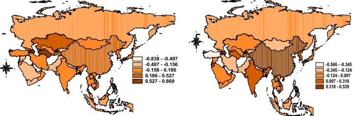
Figure a: Global Model Residuals Map. Figure b: GWR Model Residuals Map.
References
1- Abramovitz, M. (1986). Catching up, forging ahead, and falling behind. Journal of Economic History, 46, 385-406.
2- Anselin, L., Bera A.K. (1998). Spatial dependence in linear regression models with an application to spatial econometrics. in: Ullah A., Giles D.E.A. (eds.), Handbook of Applied Economics Statistics, Springer, Berlin.
p -0.838 - -0.497 -0.497 - -0.156 -0.156 - 0.186 0.186 - 0.527 0.527 - 0.869 N
E W
S
N
E W
S
3- Anselin, L. (1993). The Moran scatterplot as an ESDA tool to assess local instability in spatial association, GISDATA Specialist Meeting on GIS and Spatial Analysis (Amsterdam).
4- Anselin, L. (1988). Spatial econometrics. Kluwer Academic Publishers, Dordrecht.
5- Anselin, L. and Florax, R. J. G. M. (Eds.) (1995). New Directions in Spatial Econometrics, Berlin: Springer.
6- Anselin, L. and Rey, S. J. (1991). Properties of tests for spatial dependence in linear regression models, Geographical Analysis, 23, 112-31. 7- Arbia, G. (2006). Introductory spatial econometrics with applications to regional convergence. Springer-Verlag, Berlin.
8- Arbia, G. and Basile, R. (2005). Spatial dependence and non-linearities in regional growth behavior in Italy. Statistica. anno LXV, n. 2, 145-167. 9- Arbia, G., and Paelinck, J.H.P. (2004), Spatial econometric modeling of regional convergence in continuous time. International Regional Science Review, 26, 342-362.
10- Armstrong, H. (1995). An appraisal of the evidence from cross-sectional analysis of the regional growth process within the European Union. in: Armstrong H., Vickerman R. (eds.), Convergence and Divergence among European Union, Pion, Londres.
11- Barro, R. J. and Sala-i-Martin, X. (1997). Technological diffusion, convergence, and growth. Journal of Economic Growth, 2 (1), 1-26.
12- Barro, R.J. and Sala-I-Martin, X. (1995). Economic growth. McGraw Hill, New York.
13- Barro, R.J. and Sala-I-Martin, X. (1992). Convergence. Journal of Political Economy. 100, 223-251.
14- Barro R.J. and Sala-I-Martin X. (1991). Convergence across states and regions. Brooking Papers on Economic Activity. 1, 107-182.
16- Bernard, A.B., Durluaf, S. (1995), Convergence in international output. Journal of Applied Econometrics, 10, 97-108.
17- Bernard, A. and Jones, C. (1996). Productivity and convergence across U.S. states and industries, Empirical Economics, 21, 113-35.
18- Brunsdon, C., Fotheringham, A. S. and Charlton M.E. (1998). Spatial non-stationarity and autoregressive models. Environment and Planning, 30, 957–973.
19- Brunsdon, C., Fotheringham, A. S. and Charlton M.E. (1996). Geographically weighted regression: a method for exploring nonstationarity. Gegraphical Analysis, 28, 281-298.
20- Carlino, G. and Mills, L. (1996) .Testing neoclassical convergence in regional incomes and earnings, Regional Science and Urban Economics, 26, 565-90.
21- Cass, D. (1965). Optimum growth in an aggregative model of capital accumulation. Review of Economic Studies, 32, 233-240.
22- Debarsy, N. and Ertur, C. (2007). The European Enlargement process and regional convergence revisited: Spatial effects still matter.
23- Durlauf, S.N., Johnson, P.A. (1995), Multiple regimes and cross-countries growth behavior. Journal of Applied Econometrics, 10, 365-384. 24- Durlauf, S. N., Johnson, P. A., andTemple, J. R., 2005. Growth econometrics. In: Aghion, P., Durlauf, S. N. (Eds.), Handbook of Economic Growth. Vol. 1A. Elsevier Science, North-Holland, Amsterdam, pp. 555ñ677.
25- Ertur, C., Le Gallo, J. and Baumont, C. (2006). The European regional convergence process, 1980-1995: Do spatial regimes and spatial dependence matter?. International Regional Science Review, 29, 3-34.
27- Fotheringham, A. S., Brundson, C. andCharlton, M.E. (2003). Geographically Weighted Regression Software (version 2.0.5). Newcastle upon Tyne:NewcastleUniversity, Department of Geography.
28- Fotheringham, A. S., Brundson, C. andCharlton, M.E. (2002). Geographically Weighted Regression: The Analysis of Spatially Varying Relationships. Chichester: Wiley.
29- Fotheringham, A. S., Brundson, C. andCharlton, M.E. (1997) Two techniques for exploring non-stationarity in geographical data. Geographical Systems 4: 59–82.
30- Hansen, B. (1996), Sample splitting and threshold estimation, mimeo. 31- Koopmans, T. (1965). On the concept of optimal economic growth. In The Econometric Approach to Development Planning, Amsterdam: North-Holland.
32- Magrini, S. (2004). Regional (di)convergence. in Henderson, J.V., Nijkamp, P., Mills, E.S. and Thisse, J-F. (eds), Handbook of regional and urban economics: cities and geography.
33- Quah, D. (1997). Empirics for growth and distribution: stratification, polarization, and convergence clubs. Journal of Economic Growth, 2, 27-59. 34- Ramsey, F. (1928). A mathematical theory of saving. Economic Journal, 38 (152), 543-559.
35- Rey, S.J. (2000). Spatial empirics for economic growth and convergence. Working Papers of San Diego State University.
36- Rey, S.J. and Montoury, B.D. (1999). US regional income convergence: a spatial econometric perspective. Regional Studies. 33( 2), 143-156.
37- Sala-I-Martin X. (1996). Regional cohesion: Evidence and theories of regional growth and convergence. European Economic Review, 40, 1325-1352.
39- Solow, R.M. (1956), A contribution to the theory of economic growth, Quarterly Journal of Economics. LXX, 65-94.
40- Swan, T.W. (1956 November). Economic growth and capital accumulation. Economic Record. 32, 334-361.
41- Vaya, E. et al. (1999). Growth and externalities across economies on empirical analysis using spatial econometrics. University of Barcelona.