*Corr. Author’s Address: University of Novi Sad, Faculty of Technical Sciences, 425
Conservative-Force-Controlled Feed Drive System for Down
Milling
Tadic, B. – Vukelic, D. – Hodolic, J. – Mitrovic, S. – Eric, M.
Branko Tadic1 – Djordje Vukelic2,* – Janko Hodolic2 – Slobodan Mitrovic1 – Milan Eric1 1 Faculty of Mechanical Engineering, University of Kragujevac, Serbia
2 Faculty of Technical Sciences, University of Novi Sad, Serbia
Reviewed in this paper are the results of theoretical and experimental investigation of a novel down milling method. The method is based on controlling feed speed using conservative forces, where the active force which provides motion is the horizontal component of the cutting force. Feed motion is therefore realized without any active forces (active drive systems), while the feed speed is regulated by precision breaking of the workpiece, which is possible through hydraulic damping. In addition to the basic theoretical model of the feed drive system, the paper also presents the dynamic model of the drive system, taking into consideration fluid compressibility. Based on the model proposed, a physical instance of the feed drive system was designed, built and tested. The results of preliminary experimental investigation speak in favour of the proposed theoretical model, which enables practical application of this type of feed drive systems.
© 2011 Journal of Mechanical Engineering. All rights reserved.
Keywords: down milling, special feed drive system, continuous feed speed control, damping
0 INTRODUCTION
Milling is a basic machining process by which a surface is generated progressively by the removal of chips from a workpiece as it is fed to a rotary cutter in a direction perpendicular to the axis of the cutter [1]. Surfaces can be generated by two methods: up milling (the cutter rotates against the direction of the feed of the workpiece) and down milling (the cutter rotates in the same direction of the feed of the workpiece). Both methods have some advantages and disadvantages [2].
In the past few years major attention has been given to research of the milling process. These research works refer to various aspects such as: influence of cutting parameters on surface roughness [3] to [5], dynamic problems in milling [6] to [8], tool wear in milling operations [9] and [10], stability of milling process [11] to [13], calculations of chip thickness in milling operations [14], optimal tool geometry selection [15], optimal tool path selection [16] to [18], optimization of machining parameters in milling using geometric programming [19], optimization of machining parameters in milling using genetic programming [20], optimization of machining parameters in milling operations using genetic
algorithm [21] to [23], optimization of machining parameters in milling operations using artificial neural networks [24] and [25], optimization of machining parameters in milling operations using a combination of the genetic algorithm and artificial neural networks [26] and [27], optimization of machining parameters in milling operations using a combination of artificial neural networks and particle swarm [28].
during machining. Considering the influence of feed motion on the surface quality and tool life, an important question is whether feed speed should be kept constant during the pass of a cutter tooth through workpiece material.
Analysis of dynamic movement equations leads to a conclusion that down milling can be performed in a completely different manner. The fact that during down milling the feed speed vector remains co-linear with the horizontal component of the cutting force, leads to an idea that conservative force can be used to control feed motion. Once the motion is initiated, the active cutting force maintains feed motion. Horizontal component of the cutting force can be used as an active force. Feed speed is controlled by an adequate conservative force. In that case, feed speed is not constant but depends on the magnitude of the horizontal component of the cutting force as well as on the characteristics of passive components, which serve to arrest the workpiece. Such a solution of the feed drive allows a braking system whose reaction-time is the magnitude of a hundredth of a second (under the influence of impulse forces), resulting in a very short braking path. With this type of feed speed control, the breaking path corresponds to the tooth pitch in conventional milling. Although it satisfies stringent demands, the technical solution of the conservative-force-controlled feed drive
system is much simpler than that of conventional, mechanical systems, since braking is performed by simple hydraulic damping.
1 MODEL OF FEED DRIVE SYSTEM
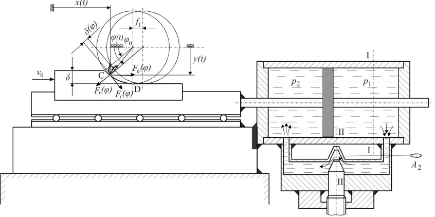
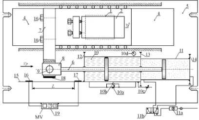
With conventional milling machines, feed drives are designed as special transmission drives (gearbox, DC motor and recirculating-ball drive, etc.) which provide constant feed motion regardless of the magnitude of resisting forces which appear during cutting. At a constant feed speed, the workpiece is moving during cutting (i.e. during the passage of cutter tooth through workpiece material). In this case, during effective cutting time (tooth engagement) the relief surface of tooth cutting wedge is additionally loaded with an external force, which provides movement for the milling machine working table and workpiece. In comparison to conventional milling, the proposed milling method has completely different basics. It uses active cutting forces to produce feed motion, while feed speed is controlled using passive hydraulic components. Conceptual design of the proposed machining method is illustrated in Fig. 1.
If the workpiece is set in motion with the initial speed ν0, at a given moment in time, the cutter, rotating at a constant cutting speed, is going to engage with a segment of workpiece material.
Horizontal component of the cutting force (Fig. 1), can be expressed by formula:
Fh( )ϕ =Ft( )sinϕ ϕ−Fr( )cosϕ ϕ, (1) where Ft(φ) and Fr(φ) are tangential and radial components of the cutting force, respectively.
The radial component of the cutting force can be expressed as:
Fr( )ϕ = ⋅K Ft( )ϕ , (2) where K is a constant which defines the ratio between radial and tangential components.
Substituting Eq. (2) into (1) gives:
Fh( )ϕ =Ft( ) sinϕ
(
ϕ− ⋅K cosϕ)
. (3) Analysis of Eq. (3) leads to a condition of movement which is derived from the following Eqs.:Fh( )ϕ >0 (4)
Ft( )ϕ >0 (5)
K<tgϕ
where φ ranges between φ0 ≤ φ ≤ 90°. Bearing in mind the cutting depths which are most frequently used in milling, it can be concluded that the condition of movement has been satisfied in most cases.
According to Fig. 1 current chip thickness is expressed as:
δ ϕ( )= ⋅f1 cosϕ, (7) where f is the movement of the workpiece (feed per tooth). Using known expressions for specific cutting resistance and tangential force, the horizontal component of the cutting force can be expressed as follows:
Fh( )ϕ =Bo
(
sinϕ−Kcos cosϕ)
ϕ(1 1− εk), (8)Bo=C b fk
(
⋅)
k−
1
1 1ε , (9)
where b is cutting width, while Bo, Ck and εk are constants depending on workpiece material.
Force Fh(φ) creates the difference in pressures (p1 – p2) within the cylinder, so that Bernoulli equations applied to cross-sections I-I and II-II give approximate equality of the following form: v 2g p g v 2g p g h
k2 1 22 2
m I I II II + ⋅ = + ⋅ + − −
∑
ρ ρ , (10)
where vk denotes piston speed (i.e. workpiece speed), p1 is pressure in the piston front-end, v2 is speed of fluid in cross-section II-II, p2 is pressure in the piston aft-end, Σhm are total losses of mechanical energy on the streaming trajectory, from cross-section I-I to cross-section II-II, g is gravitational constant and ρ is fluid thickness. All mechanical energy losses along fluid streaming path can be disregarded as lower order values in comparison with the losses in the throttling valve. From the continuity equations for the cross-sections:
ρ⋅ ⋅v Ak k = ⋅ ⋅ρ v A2 2, (11) follows the speed of fluid through the throttling valve (cross-section II-II):
v A
Akvk
2 2
= , (12)
where Ak is the active surface area of piston, A2 is the active surface area at the point of damping. Considering the surface areas ratio (Ak/A2) all the remaining losses in mechanical energy can be disregarded, compared to the losses in throttling valve, thus leading to:
h v
g h
m g m
I I II II
− −
∑
=ξ 22 ≈∑
2 , (13)
where ξg denotes mechanical energy loss coefficient. Pressure drop is determined as the function of external load, using:
∆p g p p g F g A h k ρ ρ φ ρ ⋅ = − ⋅ = ⋅ ⋅
1 2 ( ) . (14)
Substituting Eqs. (12), (13) and (14) into Bernoulli’s Eq. (10) leads to:
v g F g A A A v g A A v g k h k k k
g k k
2 2 2 2 2 2 2 2 2 2 0 + ⋅ ⋅ − − − = ( ) . ϕ ρ ξ (15)
dimensions of the hydraulic assembly, using the following expression: v F A A A k h
k k g
= ⋅
(
+)
− 2 1 1 2 2 ( )ϕ ρ ξ . (16)There are two boundary states for feed motion.
1. The first boundary state pertains to a fully blocked system, when the throttling valve is closed (A2→0), turning Eq. (16) into:
v v
F
A A
k A k
h
k k g
1 0 2 2 2 1 1 0 = = = ⋅
(
+)
− = → lim ( )ϕ ρ ε ξ , (17)where ε is an infinitely small value.
2. The second boundary state is a theoretical state in which A2 = Ak and Ak → 0, which means that:
vk A A v F
A k h g k k 2 0 2 2 = = ⋅ ⋅ → ∞ = →
lim ( )ϕ
ρ ε ξ . (18)
The first boundary state, with vk = 0, is practically achievable, and it can be proved that it is practically possible to create hydraulic design which provides continuous selection of feed speeds for all real cutting conditions. For down milling, it is the continuous selection of mean feed speed because feed speed is the function of horizontal cutting force component.
Eq. (16) can be expressed in following form:
vk =vp=R Fk h( )ϕ , (19)
where Rk, the constant of feed speed regulation, is expressed as:
R
A A
A k
k k g
= ⋅ ⋅
(
+)
− 2 1 1 2 2 ρ ξ . (20)This is called the constant of feed speed regulation as it can be set to any value from zero-up to values which fit current cutting conditions.
Feed speed vp can be defined as the first derivative of traversed path, i.e. of coordinate x in time:
v dx
dt R F
p= = k h. (21)
Using: dx dt d dt dx d dx d = ϕ =
ϕ Ω ϕ, (22)
is derived: Ωdx
dϕ =R Fk h( )ϕ , (23)
where Ω is the angular velocity of milling cutter. Based on the expression derived, it is possible to calculate total displacement of workpiece during single tooth cutting:
f dx R F d
x x k h o 1 2 1 2 1 =
∫
=∫
Ω ( ) / ϕ ϕ ϕ π (24)that is, by substituting Fh(φ) from Eq. (8) into Eq. (24), there follows:
f R
B K d
k o k o 1 1 1 2 = ⋅ ⋅
(
−)
− ∫
Ωsin cos cos
/
ϕ ϕ ϕ ε ϕ
ϕ
π . (25)
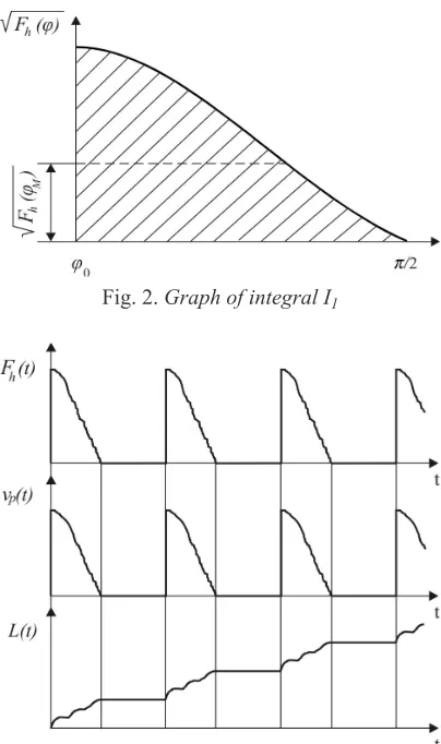
Should the value of this integral be denoted with I1, there follows:
f Rk
1= Ω I1. (26) The value of integral I1 corresponds to the area shown in Fig. 2. The size of the area in Fig. 2, i.e. the value of integral I1 can be calculated as:
I1= −
=
Fh(ϕM) π ϕo Fh(ϕ ϕM) z
2 , (27)
where φz is the angle of tooth engagement, and Fh(ϕM) denotes mean value of function
Fh( )ϕ which defines cutting conditions and has
a constant value.
By substituting Eqs. (27) to (26) the final expression, which defines displacement of workpiece during engagement of a single tooth is derived:
f R Fk h M z 1=
(ϕ ϕ)
Ω . (28)
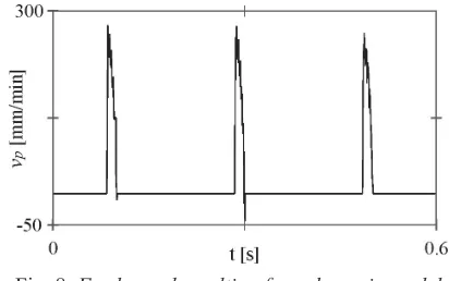
of primary motion. With this method of milling, the feed speed, vp, and feed per tooth, f1, are not constant but vary as the function of the horizontal component of the cutting force. Fig. 3 shows theoretical dependence of Fh(t), vp(t), and L(t) on the time of machining.
Fig. 2. Graph of integral I1
Fig. 3. Dependence of horizontal component of cutting force Fh(t), feed speed vp(t), and traversed
path L(t) on time t
Control of feed motion using horizontal component of the cutting force differs from conventional methods for feed motion control in milling, in the following:
• displacement of workpiece takes place only during engagement with tooth (teeth), while in the case of conventional milling the displacement takes place at a constant rate, • by regulating flow by throttling valve
continuous control of the mean feed speed
can be achieved, while the conventional gearboxes on milling machines allow this change only stepwise, and
• feed speed is variable and ranges from the selected value at point C, down to zero at point D (Fig. 1), which belongs to the machined surface.
However, it should be noted that both the conventional milling and the milling method which uses conservative forces to control feed speed, represent special cases of a more general theoretical milling method.
If, besides cutting forces, the workpiece is under the influence of an active force, Fak, which acts in the direction of feed motion, then feed speed can be calculated as:
vp =R Fk ak +F th( ) . (29)
For larger values of Fak, i.e. in cases when Fak >>Fh(t), feed speed is approximately constant, rendering this method equivalent to conventional down milling. When active forces are smaller (Fak<<Fh(t)) this milling method employs feed speed control as described above.
Previous theoretical analysis ignored the compressibility of fluid which fills the hydraulic cylinder. However, for the purpose of practical realization of conservative-force-controlled feed drive, a detailed analysis of dynamic equations was conducted, taking into account fluid (oil) compressibility.
2 DYNAMIC MODEL OF THE FEED DRIVE SYSTEM
(Fp), and elastic force which is the result of fluid compressibility (Fe).
Fig. 4. Diagram of dynamic model of feed drive system
Under the influence of the stated forces, during the finite time interval Δt, the piston shall traverse path from point P to point P2. The path PP1 traversed by the piston is proportional
to the volume of fluid passing through the throttling valve during Δt interval, while the piston displacement P P1 2 is the result of fluid
compressibility. A dynamic model of the feed drive system (Fig. 4) has two degrees of freedom. Total displacement of workpiece comprises the controlled segment PP1, which is regulated by
the damping rate, and the segment P P1 2 which
is not subject to control. The displacement P P1 2
depends on the coefficient of compressibility and the geometry of hydraulic cylinder. For the expected load level during machining, the flow speed of real fluid does not differ significantly from the flow speed of ideal fluid. Bearing this in mind, the dynamic model of feed drive can be represented by Fig. 5.
Fig. 5. Dynamic model of feed drive system
In cylinder 1 there is a real compressible fluid, while cylinder 2 contains the ideal,
incompressible fluid. The resulting force shall influence displacement along ξ and x coordinates. Force balance equation for this system is:
Fin F F F F F
e p T h ak
+ + + + + =0. (30)
Inertial force Fin represents the total system inertial force and can be expressed as:
F m d
dt m d xdt
in = 2 +
2 2
2 ξ
, (31)
where m is the total movable mass (slider, piston rod, etc.), ξ denotes piston displacement due to compression of the real-compressible fluid, while x is piston displacement allowed by the selected damping coefficient.
From the equation:
s V
dV dp
A d A L
A dF
k
k
k e
= = ⋅
⋅
1
1
ξ
, (32)
follows that the elastic force Fe equals:
F A
s L
e = ⋅k ξ, (33)
where the stiffness is defined by the ratio (Ak/ s×L), and Ak is the active piston surface area, s is oil compressibility coefficient, and L is the length of cylinder at the front of the piston at the observed moment in time. Damping force Fp can be determined based on Eq. (19). The magnitude of this force retains its form of dependence, and can be calculated as function of piston speed:
F R
dx dt
dx dt p
k
= ⋅
⋅
1 2 sgn , (34)
F R dx
dt
dx dt p = r⋅
⋅
2
sgn , (35)
where Rr is reciprocal value of the regulation constant Rk given in Eq. (20), and dx/dt is the speed of piston due to flow of fluid through the throttling valve.
Damping force Fp is the conservative force used to control the down milling feed. In conventional milling this force does not exist, while feed is controlled in a completely different way.
linear roller guides) for the most part, the friction force can be neglected. The magnitude of active force Fak can be chosen arbitrarily, while the horizontal component of the cutting force, as a smooth function of time, can be defined as:
F t F t t
t t K
h t
( ) sin sin
sin sin cos max = −
(
+)
(
)
⋅ ⋅ + Φ Ω Φ Ω Ω Ω β βssinΩ t
(
)
(36)
where Φ is Heaviside function, and Ftmax is the maximum value of the tangential component of the cutting force.
Based on the forces defined, the differential equation of displacement can be set:
m d
dt m d xdt
A sL
R dx dt
dx
dt F t F
k r h 2 2 2 2 2 ξ + + ξ+ + ⋅ = +
sgn ( ) aak.
(37)
There is a following relationship between the elastic force Fe and damping force Fp:
A
sL R dxdt
dx dt k r ξ = ⋅ 2
sgn , (38)
from which the following is derived:
A s L
d
dt R dxdt
d x dt k r ⋅ = ξ
2 22 , (39)
while the acceleration follows from:
d x dt
A s L R
d dt k r 2 2 1 2 = ⋅ ⋅ ⋅ξ ξ . (40)
For both senses of motion the same damping rate was adopted, i.e.:
Rr(x<0) = Rr(x > 0), (41)
although a solution can be found for other damping rates. By substituting both Eq. (40) and relationships between elastic and damping forces into Eq. (37), a nonlinear differential equation is derived:
m d dt
m A
s L R d
dt A
s L F t F
k r k h ak 2 2 2 2 ξ ξ ξ ξ + ⋅ ⋅ ⋅ + ⋅ ⋅ = ( )+ (42)
The problem is now reduced to defining the law of motion ξ(t). Analysis of differential Eq. (37) leads to the conclusion that the magnitude of displacement ξ depends, among other factors, on the damping rate Rr. Observing the boundary condition of the system when the throttling valve is completely blocked (closed), it can be concluded that the displacement x equals zero, reducing Eq. (37) to the following form:
m d dt
A
s Lk F th Fak
2
2
ξ + ξ
⋅ = ( )+ . (43)
In this boundary case, the total work of external forces Fak and Fh(t) shall be spent on fluid compression in cylinder 1. The magnitude of this work depends on the magnitude of damping rate Rr, so ξ - which is derived from Eq. (43) - has the largest possible value. Thus, the law by which ξ(t) changes in time can be expressed by:
m d dt
A
s Lk Z F th Fak
2
2
ξ + ξ
⋅ = ( )+ , (44) where Z is an unknown constant. Eq. (44) has an analytical solution, which is given here in its final form:
ξ t A t ω t B t ωt
C t t D t t E
( )
=( )
+( )
++
( )
+( )
+1 1
1 2 1 2 1
cos sin
sin Ω sin Ω
( )
tt , (45)where Ω is forced frequency, ω is eigenfrequency. Eigenfrequency is given as:
ω = ⋅ ⋅
A
s L mk , (46)
while the remaining parameters follow from:
h t F Z
m t
t t
1
( )
=− ⋅ ⋅
(
)
−(
+)
max sin sin sin β β Φ Ω Φ Ω , (47) h F mak2= , (48)
C t1 2 h t1 2
0 5 4
( )
=( )
−
,
ω Ω , (49)
D t1
( )
= h t K21 4 2( )
−
ω Ω , (50)
E t1 h2 D t
2 1 2
2
( )
= − Ω( )
B t1
( )
= −2ΩC t1( )
ω , (52)
A t s L
Ak Fak E t
1
( )
= 1⋅ −
( )
. (53)
The law of change ξ(t), defined by Eq. (45) and a constant Z = 0.5, identically satisfy Eq. (41) for any m, Ak, s, L, Rr and forces Fh(t), and Fak.
The speed of fluid compression (v2) in the hydraulic cylinder is calculated as a derivative of displacement ξ(t) in time:
v t d
dt
A t t B t t
C t t D
2
1 1
1 1
2 2
( )
= == −
( )
+( )
++
( )
+ξ
ωsinω ωcosω
cos
Ω Ω
( )
tt Ωsin 2Ωt, (54)while the controlled segment of speed (v1) can be calculated as:
v dx
dt
A s L Rk r
1= = ⋅ ⋅ ξ . (55)
Workpiece feed speed equals the sum of v1 and v2, that is:
vp= +v v1 2, (56) while the total displacement of workpiece equals:
x tp t x t t v t dt
t
( )
=ξ( )
+( )
=ξ( )
+∫
1( )
0
. (57)
Fig. 6. Feed speed resulting from dynamic model with following inputs Ftmax = 3000 N; Fr/Ft = 0.7; s = 3×10⁻¹⁰ m2/N; W = 31.4 s-1; m = 50 kg; L = 0.2 m; Ak = 0.0144 m2, Fak = 0 N;
Rr = 105 N1/2s/m, δ = 5 mm; D = 100 mm Based on the equations given above, a software application was made which allows
calculation of current feed speeds and workpiece displacements, for various input values.
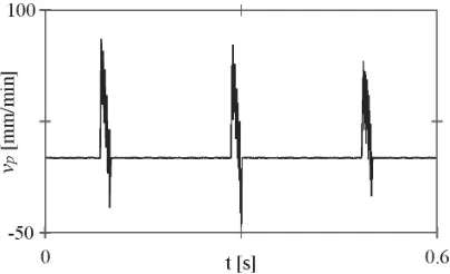
Shown in Figs. 6 and 7 are diagrams of boundary feed speeds which are the result of two different damping rates Rr = 105 N1/2s/m (Fig. 6), and Rr = 1010 N1/2s/m (Fig. 7).
Fig. 7. Feed speed resulting from dynamic model with following inputs Ftmax = 3000 N; Fr/Ft = 0.7; s = 3×10⁻¹⁰ m2/N; W = 31.4 s-1; m = 50 kg; L = 0.2 m; Ak = 0.0144 m2, Fak = 0 N; Rr = 1010
N1/2sm-1, δ = 5 mm; D = 100 mm
It should be noted that higher damping rates Rr (Fig. 7) prohibit machining by the proposed technology. Namely, there is an area of damping rates Rr and stiffness (Ak/s×L) which provides sufficient displacement of workpiece. For particular stiffness, the level of damping rate Rr can be selected such as to allow cutting with feed speeds common to milling, which is shown in Figs. 8 to 10.
Fig. 8. Feed speed resulting from dynamic model with following inputs Ftmax = 3000 N; Fr/Ft = 0.7;
Fig. 9. Feed speed resulting from dynamic model with following inputs Ftmax = 3000 N; Fr/Ft = 0.7;
s = 3×10⁻¹⁰ m2/N; W = 31.4 s-1; m = 50 kg; L = 0.2 m; Ak = 0.0144 m2, Fak = 0 N; Rr = 5×10⁸ N1/2sm-1, δ = 5 mm; D = 100 mm
Fig. 10. Feed speed resulting from dynamic model with following inputs Ftmax = 1000 N; Fr/Ft = 0.7;
s = 3×10⁻¹⁰ m2/N; W = 31.4 s-1; m = 50 kg; L = 0.2 m; Ak = 0.0144 m2, Fak = 2000 N; Rr = 109 N1/2sm-1, δ = 5 mm; D = 100 mm
Fig. 11. Feed speed resulting from dynamic model with following inputs Ftmax = 3000 N; Fr/Ft = 0.7;
s = 3×10⁻¹⁰ m2/N; W = 31.4 s-1; m = 50 kg; L = 0.2 m; Ak = 0.0144 m2, Fak = 2000 N; Rr = 109 N1/2sm-1, δ = 5 mm; D = 100 mm
If, in addition to the horizontal component of the cutting force, active force Fa is also acting upon piston rod, then the proposed feed drive dynamically behaves similarly to the conventional one. Fig. 11 shows the law of feed speed change in case of an active force of higher magnitude.
Total displacement of the workpiece, defined by Eq. (57), also comprises displacement component ξ which is not subject to control. The magnitude and law of change of displacement ξ(t) depend on the following parameters: the stiffness of hydraulic assembly (Ak/s×L), magnitude and ratio between the radial and tangential cutting force (Fr, Ft, K), mass of movable feed drive components (m), cutter diameter (δ), cutting depth (D), and angular speed of the cutter (Ω). For particular values of these parameters and within some period of cutting, the displacement ξ reaches its maximum. It is of utmost importance to choose such construction parameters Ak, s, L, and m, which would for the expected magnitudes of cutting force components allow the uncontrollable ξ to be kept at insignificant level. This can be realized by increasing the stiffness of the hydraulic assembly. Values of stiffness (Ak/s×L) and mass (m) should be chosen in such a mannerthat given real machining conditions system oscillations are kept out of the resonance area.
The magnitude of resonant frequency is defined by:
Ω =
⋅ ⋅
1 2
A
s L mk . (58)
L = 0.2 m, and active piston area Ak = 0.014 m2. For the given machining conditions, the maximum value of uncontrollable displacement ξ(t) does not overstep 3 mm (Figs. 12 and 13), which makes it practically possible to establish control from zero to the desired value by shifting x.
Fig. 12. Dependence of displacement ξ on cutting time interval, at angular speed Ω = 10 s-1
Fig. 13. Dependence of displacement x on cutting time interval, at angular speed Ω = 50 s-1
3 DESIGN OF FEED DRIVE SYSTEM
The results of the theoretical analysis from previous sections were used to design a physical prototype of the feed drive system for down milling operations. This feed drive system establishes control over the feed motion based on the horizontal component of the cutting force. Feed drive components are designed in such a way that they allow continuous shift of feed speed within the vp = 0 to 500 mm/min interval, at the maximum value of the horizontal component of the cutting force Fhmax < 10000 N.
chosen damping rate and machining parameter. Hydraulic cylinder is equipped with a throttling valve (10c) which controls oil feed to the cylinder. During feeding, the throttling valve (10a) is open due to alternate movements of piston rod and air let-off. In order to eliminate negative effects of trapped air in the hydraulic cylinder, oil is fed under pressure, which is controlled by the pressure gage (10d). The feed drive system described is a module independent from the original machine tool feed drive (milling feed drive system is shut off during entire machining process). The milling machine worktable, in this case, assumes the role of a stable platform to which a module is attached which assumes the function of the drive system. The feed drive system is shown in Fig. 15.
Fig. 14. Schema of the proposed feed drive system
Fig. 15. Feed drive system mounted on the milling machine worktable
4 TESTING OF FEED DRIVE SYSTEM
Prior to experimental investigation, the feed drive system was tested. In addition to testing the geometric accuracy of the moving components of the feed drive system, and checking the stiffness of joints, the relationship between feed speed and axial force was also determined. The axial force exerted by compressed air in the pneumatic cylinder simulates the horizontal component of the cutting force, while the table speed is calculated as the ratio between L and time of cutting t (Fig. 14). By varying the input air pressure one a range of values for axial force (Fai) and time (ti) for which the table travels along path (L) is derived. The active force (Fa) is calculated based on the pressure which reads on the manometer of the air service unit and the diameter of the pneumatic cylinder. The described method was used with various damping rates, producing the experimental data shown in Table 1.
Statistical analysis of experimental data by regression analysis with the basic function of following form:
(Fak – C) = Rr × v2 (59) results with the regression equations of high degree of correlation (Table 2). In Eq. (59) (Fak – C) represents effective force which performs the movement. Namely, the constant C includes friction forces and other opposing forces which are always present, while the member Rr × v2 defines quadratic dependency of feed speed on effective force. This relationship (Rr × v2) was derived from a set of Bernoulli equations within the theoretical investigation. Regression equations and correlation coefficients confirm this relationship (Table 2). Given in Table 2 are feed speeds and axial forces, derived by regression equations, as well as the percent deviations between the measured and calculated values. The differences in constant C could be attributed to the influence of feed speed on the magnitude of friction force. The decrease of friction force is due to higher feed speeds, which is confirmed by statistical analysis.
5 PRELIMINARY EXPERIMENTS
the feed drive, preliminary experiments were conducted. Extensive follow-up experimental investigation is planned in the future to determine the quality of a number of machining parameters derived by the novel method, as well as to compare them with those obtained by conventional methods.
Preliminary experimental investigation was conducted under following conditions:
• The machining was performed using feed drive of a universal milling machine PGU–3. • Workpiece material: C1530, hardness 190 to
205 HB, with 0.44% C; 0.18% Si; 0.27% Mn; 0.011% S; <0.010% P,
• Cutter: standard end mill 80X10X27N, • Cutting regime parameters were as follows:
cutting speed 22.6 m/min, feed speed 112.8 mm/min, cutting depth 1 mm, cutting width 10 mm.
The following parameters were monitored during the experiment:
Table 1. The results of measurement for pressure p, time t, the calculated force Fa and feed speed vp
Damping rate Rr1 Damping rate Rr2
p
[bar] [N]Fak [s]t [mm/min]vp [bar]p [N]Fak [s]t [mm/min]vp
1.5 1062 140 64.3 1 715 50 180
2 1430 86 104.7 1.5 1052 32 281.3
2.5 1788 65 138.5 2 1430 24 375
3 2145 52 173 2.5 1788 19 473.8
3.5 2502 44 204.6 2.9 2073 17 529.5
4 2860 39 230.7 3.5 2502 15 600
4.4 3146 35 257.3 4 2860 13 692.5
- - - - 4.4 3146 12 750
Table 2. Results of statistical analysis
Damping rate Rr1 Damping rate Rr2
vp
[mm/min] F[N]ak1 [%]DF [mm/min]vp F[N]ak2 [%]DF
64.3 1204 14.2 180 872 -15.7
104.7 1430 8.5 281.3 1083 -2.1
138.5 1702 8.6 375 1361 6.8
173 2058 8.7 473.8 1741 4.6
204.6 2452 4.9 529.5 1994 7.8
230.7 2828 3.1 600 2355 14.7
257.3 3258 -11 692.5 2896 -3.6
- - - 750 3272 -12.8
Regression equation Fak-106.7=3.31×10⁻³×vp2
r = 0.993, s = 10.1 Regression equation Fak-72.5=4.53×10 -4×vp2 r = 0.992, s = 11.3
Fig. 17. Wear curve for characteristic cutter teeth in dependence of cutting time
Fig. 18. Profile of machined surface after 31.8 minutes of cutting
Fig. 19. Profile of machined surface after 347.6 minutes of cutting
• Mean flank wear on the four characteristic cutter teeth. As an example, in Fig. 16 images of worn teeth generated on Meiji Techno MC50 microscope are shown. Based on the measured flank wear, a diagram of wear
curves is given in Fig. 17 for the characteristic cutter teeth,
• The profiles of the machined surface were taken after two cutting intervals, using Taylor Hobson – Talysurf 6 apparatus. The profiles are shown in Figs. 18 and 19.
6 CONCLUSION
The proposed theoretical model implicates the practical possibility of controlling feed motion in down milling by hydraulic damping, where the horizontal component of the cutting force is used to actuate motion. The theoretical model proposed should be taken as a fundamental model, which clearly implies the possibility of practical machining as described in this paper. Based on the proposed model, which can be conditionally treated as a static model, a dynamic testing of the feed drive system was also performed. The results of dynamic modelling show that the horizontal component of the cutting force can be successfully used as the active force in down milling feed motion. The results of dynamic modelling also show that the hydraulic damping allows a very precise control of the down milling feed motion. Testing of the physical prototype of the feed drive system also allowed preliminary experimental investigation to be performed on a real machining system.
The results of preliminary experimental investigation allow the following conclusions: • Down milling is possible according to the
proposed method, which completely verifies the proposed theoretical model.
• Tool life and surface quality obtained by the proposed method are of the same order of magnitude as those obtained by conventional machining methods.
7 REFERENCES
[1] Stephenson, D.A., Agapiou, J.S. (2006). Metal Cutting Theory and Practice, 2nd ed. CRC Press, Boca Raton.
[2] Boothroyd, G., Knight, W.A. (2006). Fundamentals of machining and machine tools, 3rd ed. CRC Press, Boca Raton.
[3] Sai, K., Bouzid, W. (2005). Roughness modeling in up-face milling. The International Journal of Advanced Manufacturing Technology, vol. 26, no. 4, p. 324-329.
[4] Davim, J.P., Clemente, V.C., Silva, S. (2009). Surface roughness aspects in milling MDF (medium density fibreboard). The International Journal of Advanced Manufacturing Technology, vol. 40, no. 1-2, p. 49-55.
[5] Mansour, A., Abdalla, H. (2002). Surface roughness model for end milling: a semi-free cutting carbon casehardening steel (EN 32) in dry condition. Journal of Materials Processing Technology, vol. 124, no. 1-2, p. 183-191.
[6] Miao, J.C., Chen, G.L., Lai, X.M., Li, H.T., Li, C.F. (2007). Review of dynamic issues in micro-end-milling. The International Journal of Advanced Manufacturing Technology, vol. 31, no. 9-10, p. 897-904.
[7] Liu, X., Cheng, K. (2005). Modelling the machining dynamics of peripheral milling. International Journal of Machine Tools & Manufacture, vol. 45, no. 11, p. 1301-1320. [8] Altintas, Y., Montgomery, D., Budak, E.
(1992). Dynamic peripheral milling of flexible structure. Journal of Engineering for Industry, vol. 114, no. 2, p. 137-145.
[9] Zeng, W., Jiang, X., Blunt, L. (2009). Surface characterisation-based tool wear monitoring in peripheral milling. The International Journal of Advanced Manufacturing Technology, vol. 40, no. 3-4, p. 226-233.
[10] Xu, C., Chen, H., Liu, Z., Cheng, Z. (2009). Condition monitoring of milling tool wear based on fractal dimension of vibration signals. Strojniški vestnik ‒ Journal of Mechanical Engineering, vol. 55, no. 1, p. 15-25.
[11] Mann, B.P., Insperger, T., Bayly, P.V., Stepan, G. (2003). Stability of up-milling and
down-milling, part 2: experimental verification. International Journal of Machine Tools & Manufacture, vol. 43, no. 1, p. 35-40.
[12] Zhao, M.X., Balachandran, B. (2001). Dynamics and stability of milling process. International Journal of Solids and Structures, vol. 38, no. 10-13, p. 2233-2248. [13] Altintas, Y., Budak, E. (1995). Analytical
prediction of stability lobes in milling. CIRP Annals - Manufacturing Technology, vol. 44, no. 1, p. 357-362.
[14] Wan, M., Zhang, W.H. (2006). Calculations of chip thickness and cutting forces in flexible end milling. The International Journal of Advanced Manufacturing Technology, vol. 29, no. 7-8, p. 637-647.
[15] Kumar Reddy, N.S., Rao, P.V. (2005). Selection of optimum tool geometry and cutting conditions using a surface roughness prediction model for end milling. The International Journal of Advanced Manufacturing Technology, vol. 26, no. 11-12, p. 1202-1210.
[16] Chu, C.H, Chen, J.T. (2006). Tool path planning for five-axis flank milling with developable surface approximation. The International Journal of Advanced Manufacturing Technology, vol. 29, no. 7-8, p. 707-713.
[17] Park, S.C., Choi, B.K. (2000). Tool-path planning for direction-parallel area milling. Computer-Aided Design, vol. 32, no. 1, p. 17-25.
[18] Balič, J., Korošec, M. (2002). Intelligent tool path generation for milling of free surfaces using neural networks. International Journal of Machine Tools & Manufacture, vol. 42, no. 10, p. 1171-1179.
[19] Sonmez, A.I., Baykasoglu, A., Dereli, T., Filiz, I.H. (1999). Dynamic optimization of multi-pass milling operations via geometric programming. International Journal of Machine Tools & Manufacture, vol. 39, no. 2, p. 297-320.
[21] Dereli, T., Filiz, I.H., Baykasoglu, A. (2001). Optimizing cutting parameters in process planning of prismatic parts by using genetic algorithms. International Journal of Production Research, vol. 39, no. 15, p. 3303-3328.
[22] Palanisamy, P., Rajendran, I., Shanmugasundaram, S. (2007). Optimization of machining parameters using genetic algorithm and experimental validation for end-milling operations. The International Journal of Advanced Manufacturing Technology, vol. 32, no. 7-8, p. 644-655.
[23] Čuš, F., Milfelner, M., Balič, J. (2006). An intelligent system for monitoring and optimization of ball-end milling process. Journal of Materials Processing Technology, vol. 175, no. 1-3, p. 90-97.
[24] Župerl, U., Čuš, F., Muršec, B., Ploj, T. (2006). A generalized neural network model of ball-end milling force system. Journal of Materials Processing Technology, vol. 175, no. 1-3, p. 98-108.
[25] Palanisamy, P., Rajendran, I., Shanmugasundaram, S. (2008). Prediction of tool wear using regression and ANN models in end-milling operation. The International Journal of Advanced Manufacturing Technology, vol. 37, no. 1-2, p. 29-41.
[26] Tansel, I.N., Ozcelik, B., Bao, W.Y., Chen, P., Rincon, D., Yang, S.Y., Yenilmez, A. (2006). Selection of optimal cutting conditions by using GONNS. International Journal of Machine Tools & Manufacture, vol. 46, no. 1, p. 26-35.
[27] Ozcelik, B., Oktem, H., Kurtaran, H. (2005). Optimum surface roughness in end milling Inconel 718 by coupling neural network model and genetic algorithm. International Journal Advanced Manufacturing Technology, vol. 27, no. 3-4, p. 234-241.