of peer-reviewed research and commentary in the population sciences published by the Max Planck Institute for Demographic Research Konrad-Zuse Str. 1, D-18057 Rostock·GERMANY www.demographic-research.org
DEMOGRAPHIC RESEARCH
VOLUME 15, ARTICLE 12, PAGES 347-400
PUBLISHED 7 NOVEMBER 2006
http://www.demographic-research.org/Volumes/Vol15/12/ DOI: 10.4054/DemRes.2006.15.12
Research Article
Trajectories and models of individual growth
Arseniy S. Karkach
c
°2006 Karkach
This open-access work is published under the terms of the Creative Commons Attribution NonCommercial License 2.0 Germany, which permits use, reproduction & distribution in any medium for non-commercial purposes, provided the original author(s) and source are given credit.
1 Introduction 348
2 Growth patterns in different phyla 352
3 Mathematical description of growth 357
3.1 Typically observed patterns of growth 359
3.2 Growth curves as empirical models 359
3.2.1 Curves for determinate growth 360
3.2.2 A curve for indeterminate growth 367
3.2.3 Multiphasic growth curves 367
3.2.4 Polynomial growth curves 368
3.2.5 A description of human growth 368
3.2.6 A description of cattle growth 371
3.3 Theories and mechanistic models of growth 371
3.3.1 A model of von Bertalanffy 371
3.3.2 The theory of growth of Turner et al. 373 3.3.3 Park’s theory of animal feeding and growth 373 3.3.4 The theory of Dynamic Energy Budgets of Kooijman et al. 373 3.3.5 The general model of ontogenetic growth of West et al. 375
3.4 Selecting the growth model 375
4 A comparison of growth between species 377
4.1 Allometry and scaling relationships 377
4.2 Animal-plant unification 379
4.3 Growth and conservation laws 380
5 What shapes the trajectories of growth? 381
6 Problems and prospects 386
7 Acknowledgements 387
research article
Trajectories and models of individual growth
Arseniy S. Karkach1
Abstract
It has long been recognized that the patterns of growth play an important role in the evo-lution of age trajectories of fertility and mortality (Williams, 1957). Life history studies would benefit from a better understanding of strategies and mechanisms of growth, but still no comparative research on individual growth strategies has been conducted.
Growth patterns and methods have been shaped by evolution and a great variety of them are observed. Two distinct patterns – determinate and indeterminate growth – are of a special interest for these studies since they present qualitatively different outcomes of evolution. We attempt to draw together studies covering growth in plant and animal species across a wide range of phyla focusing primarily on the noted qualitative features. We also review mathematical descriptions of growth, namely empirical growth curves and growth models, and discuss the directions of future research.
1
Introduction
The ontogenetic growth of an individual is intuitively understood to be an increase in the size of the whole organism or parts of it with age. But the very “natural” notion of growth is, in fact, very difficult to define. Living organisms are complex systems, consisting of parts that often grow at different rates and displaying different patterns. Some parts of the body may grow faster than others, some may stop growing at a certain stage while others continue to grow, and organs may grow “on demand” during regeneration. The cells of an organ may divide continuously throughout an organism’s life, replacing aging cells and producing cell turn-over in the tissues; still the body size may remain constant.
Growth is coordinated by a program of ontogenetic development that allows for vari-ability in the development rates and sizes in order to adapt to environmental conditions. Size and growth rates are subject to evolutionary optimization and constraints. On the one hand, larger size usually leads to greater mating success, greater fertility, lower vul-nerability to environmental hazards, and thus lower mortality. On the other, growth needs resources, and trades-off with other traits.
Studies on growth and maintenance shed light on the problem of senescence. Most organisms experience cell turn-over in most tissues. Some organisms (e.g. hydra) appar-ently escape senescence due to a quick turn-over of cells (Martínez, 1998).
Growth and body size are strongly related to other traits and fitness. Research on ex-tant species showed a strong statistical relationship between body mass and a remarkable variety of biological features (Smith, 1996).
Measures of growth
Growth as an increment in size can be measured in many different ways, each having ad-vantages and drawbacks. An increase in mass or volume often can be measured easily, but may be only indirectly related to growth as increase in biomass. Organisms may change in content of water or fat, in mass and volume, but this is not considered as growth. To account for such changes, measurements of dry and fat-free mass have been devel-oped. However, these measurements are often destructive. Non-destructive methods of body composition measurement include X-ray absorptiometry, electrical impedance, and imaging techniques (see (Heymsfield et al., 2005) for a comprehensive review).
The growth of small multicellular organisms can be measured as an increase in the number of cells. In certain cases, the volume and mass of cells may change without a corresponding change in cell numbers (e.g. during muscle training).
It seems impossible to propose a single definition and measure of growth suitable to all applications. Different studies employ different measures of size and growth, such as mass and volume, and different linear measurements, such as dry, fat-free mass, bone-free mass, and cell counts. But the different measures are often incompatible with each other, and conversion between them often includes unknown factors, such as shape, body density, fat, bone or water contents. This is why caution should be taken when comparing growth measured in different ways (an example of such difference is illustrated in Fig-ure 8).
Length, volume, and shape
The volume of an organism is related to its linear measures in different ways, depending on the construction of the organism. Several main types of constructions can be distin-guished. In isomorphically growing organism, all linear dimensions change proportion-ally, and volumeV is related to any of its linear measures, LasV =αL3, whereαis a shape parameter. If the shape does not change,α=const. Typically, organisms change shape as they increase in size, so the value of shape parameterαchanges. Some organ-isms, having the shape of sheets, films, and flat bodies with a constant, but small height (such as leaves), grow in two dimensions. In such organisms,V =αL2. Some organisms have the shape of sticks or rods and grow only in one dimension. The relation between the linear measure and volume in them isV =αL. The volume is proportional to the surface area in the latter two types. A detailed description of the relations between volume and linear size be found in (Kooijman, 2000, chapter 2.2.2).
Methods of growth
Animals and plants are constituted of parts that, during ontogeny, may grow at different rates and according to different patterns. For example, tree branches and tree roots can grow indefinitely, whereas leaves and flowers show a clear determinate pattern. Several “ways” or methods of growth can be distinguished (after Raup and Stanley (1978)):
Accretion – adding new material to an existing skeleton. This kind of growth is typical for mollusks, trees (growth rings), fish scales, and the teeth of some vertebrates.
accompanied by moulting. In such organisms, the skin or exoskeleton protects the organ-ism, but also limits expansion; thus it is periodically replaced with a new, larger skin or exoskeleton.
Modification – the re-formation and re-shaping of the original material as size in-creases. Vertebrate bones grow in this fashion.
Often, a mixture of growth patterns is observed. Trilobites add segments while molt-ing. Echinoderm plates accrete and new ones are also added; cephalopods both accrete and add walls between chambers.
Growth can be continuous or discontinuous. Examples of discontinuous growth are clams in the gulf of California. Their growth starts in late March, speeds up in spring and early summer, slows or stops, speeds up again, and then stops in late November. Discontinuous, pulsed growth can be observed in perennial organisms – they grow rapidly in the beginning of the season and decrease or shut down growth and other metabolic activities between the seasons to survive.
The so-called “catch-up” growth is observed in organisms with a genetically deter-mined target size. When early life conditions (usually the lack of food) disfavor the growth of an individual in comparison to others, the latter may catch-up with their more “lucky” competitors later in life. Such growth pattern can be found in birds.
“Growth on demand” — the regeneration observed both in determinate and indeter-minate growing organisms (e.g. wound closing; liver regeneration in humans; tail regen-eration in reptiles; leg, eye, and tail regenregen-eration in axolotl (Tanaka, 2003)) can also be observed.
Qualitative types of growth
Growth patterns are traditionally classed in two groups: determinate and indeterminate ones. They have two principally different features, presumably demonstrating different optima of life history evolution.
Determinate growth is usually defined as growth that stops when an organism reaches a certain size. Usually growth stops during the reproductive stage. Indeterminate growth is defined as growth that continues past maturation and may continue to the end of life (Heino and Kaitala, 1999).
Determinate growth is observed in bacteria and other unicellular organisms, all birds, some plants, fish, insects, and most mammals. They rapidly grow to a pre-defined adult size, at which physical growth stops, and then mature at a characteristic adult size. Some organisms (such as the Nematode worm, the fruit fly D. melanogaster, C. capitata) have a posmitotic adult stage (imago), at this stage cells do not divide and there is no growth.
many modular animals such as corals and sponges, and “lower” vertebrate taxa, such as most fish, amphibians, and reptiles (lizards and snakes). It is also found in perennial plants and most trees (Lika and Kooijman, 2003; Vaupel et al., 2004). The best studied animals that exhibit indeterminate growth are sea urchins (Strongylocentrotus) and salmon. The adult size of these organisms depends largely on the environmental conditions they live in. In theory, they can get as large as their environment and diet allow.
The literature commonly notes that all mammals and even “all higher vertebrates” grow determinately. But male eastern and western grey kangaroos, wallabies, pademelons and swamp wallabies, American bisons, giraffes, African and Indian elephants, mule deer, and white-tailed deer seem to grow after maturity and throughout their life and hence to have have indeterminate growth. The females of these species can grow determinately. Thus indeterminate growth can also be enjoyed by higher organisms.
Both growth strategies can occur even among closely related taxa: cladocerans show indeterminate growth (Daphnia magna can grow by a factor of two in length, i.e. a fac-tor eight in volume, during the reproductive period), while copepods show determinate growth (Kooijman, 2000, p. 293), both being members of the phylum Arthropoda, class Crustacea. Some plant species (such as tomatoes, lablab bean) show both types of growth, depending on environmental conditions or genetic variations.
This review is largely biased towards reviewing these qualitative growth types in dif-ferent organisms. Some comments can be made on the definitions of growth patterns.
Is indeterminate growth never ending?
The definition of indeterminate growth may be confusing and may mislead to think that indeterminate growers never cease to grow. Certainly, nothing in nature can grow with-out limit. The maintenance of a larger body requires more energy, so the production of food and the capacities of organismal systems (e.g. respiratory, digestive) should increase accordingly. Sooner or later, various limitations will stop growth. Organisms in natural populations die early because they are subject to predation and environmental hazards. In favorable laboratory conditions, they usually live longer. Indeterminate growth, i.e. growth to which no end is observed during the natural lifespan, may stop if the organism had a chance to live longer. The main difference between the definitions is that indeter-minate growth does not stop at, or soon after, reaching maturity, so organisms are able to increase their size-related reproduction capacity with time.
Determinate growth after sexual maturity
processes that may take considerable time. In determinately growing organisms (such as humans), growth may not stop at the age of sexual maturity but continue for some time. For example, growth in humans does not cease entirely after sexual maturity is reached, but it does slow down significantly. By the time of sexual maturity, humans attain most of their adult height. Girls may add some height, as much as 5 cm, over the next two years. For boys, there is no such a clear end point, though there are also indications of full sexual maturity. Again, there may be some small additional growth in height after they reach this stage of development (see Figure 8).
Different parts of the organism can grow with different patterns
Consider a perennial long-living plant, a tree. The tree trunk constitutes the main, critical part of the tree; a serious damage to it will lead to death. The trunk grows indeterminately, gaining height and width, and acquiring rings. The roots also grow indeterminately to support the nourishment needs of the trunk and to provide stable support. Leaves, by con-trast, grow at the beginning of each season, their growth is determinate and their size well defined. They provide the tree with photosynthesis and gas exchange. The leaves tear and wear and have no chance of surviving the cold season. So, at the end of the season, the tree removes water and nutrients from the leaves and sheds them. The cycle is repeated in the next season. Flowers and fruits of trees also grow determinately.
Growth, maintenance, and turnover
Living tissues age. In many cases, the lifespan of single cells is much shorter than that of tissues or the whole organism. To provide greater longevity, tissues undergo a constant process of turn-over, including the breaking-down of old and damaged components and the synthesis of new ones. Growth from the energetic, metabolic point of view may be considered as an excess of build-up over the break-down of tissues. This view was first proposed by Pütter (1920) and developed by Bertalanffy (1941, 1957) in his model of growth (see 3.3.1).
Many tissues in an adult human are renewed approximately every seven years; this corresponds to a synthesis of 13% of biomass yearly; the rate is comparable only to fast growth in childhood. So, it is not unrealistic to assume that turnover expenses, usually included in maintenance, are comparable to or greater than the expenses on growth itself.
2
Growth patterns in different phyla
Table 1: Growth patterns in different phyla
Phyla Determinate Indeterminate
Kingdom Protista Rhizopods (e.g. Amoeba (Amoeba
proteus) (Prescott, 1957))
Kingdom Fungi Yeast (Saccharomyces cerevisiae,
Saccharomyces carlsbergensis)
(Berg and Ljunggren, 1982), most mushrooms
Hornwort
Kingdom Plantae1 Trees (leaves), lablab bean (Lablab
purpureus), tomato (certain species,
mostly early ripening), white lupin (Lupinus albus L.) (autumn-sown type) (Huyghe, 1997), soybeans (Robinson and Wilcox, 1998)
Trees (branches, trunks), peren-nial plants (primary bodies), roots, lablab bean (Lablab purpureus), tomato (certain species), white lupin (Lupinus albus L.) (spring-sown type) (Huyghe, 1997), soy-beans (Robinson and Wilcox, 1998)
Kingdom Animalia
Phylum Cnidaria Hydra (Martínez, 1998) Many benthic marine inverte-brates (Sebens, 1977)
Phylum Nematoda Nematode worm (Caenorhabditis
el-egans) (Lee, 2002)
Subkingdom
Meta-zoa Phylum Annel-ida
Segmented worm Pristina leidyi
(Bely and Wray, 2001), (Dorresteijn and Westheide, 1999)
Phylum Mollusca Snails (class Gastropoda), strom-bids (gastropods of the family
Strom-bidae)
Long-lived freshwater bivalves, clams, freshwater mussels (Heino and Kaitala, 1999; Hanson et al., 1989; Jokela, 1997)
Phylum
Echinoder-mata
Sea urchins
(Strongylocentro-tus) (Stephens, 1972; Gage and
Tyler, 1985) Phylum
Arthro-poda2 Class In-secta
Insects with terminal moult, fixed number of instars (growth stages) – usually those with wings (most in-sects)
Insects with no terminal moult and no fixed number of instars (aptery-gote insects)3
Class Crustacea Copepods (Kooijman, 2000), fe-males of Chionoecetes crabs (Stone, 1999)
Phyla Determinate Indeterminate Phylum Chordata,
Subphylum Verte-brata, fish6
Some fish species Many species of teleost fish (Weath-erley and Gill, 1987b), zebrafish (Danio rerio) (Kishi et al., 2003),
Brachyrhaphis rhabdophora (Poecili-idae family)7and other poeciliid fish, salmonids (Salmonidae) – salmon, trout, Atlantic salmon (Grant et al., 1998; Purdom, 1993), Yellow perch (Huh, 1975; Malison et al., 1985) Class Reptilia8 Blanding’s Turtles (Emydoidea
blandingii) (Congdon et al., 2001,
2003)
Painted Turtles (Chrysemys
picta) (Congdon et al., 2001, 2003)9, other tutrtles, snakes, lizards
Class Aves (birds) All birds (Starck and Ricklefs, 1998; O’Conner, 1984)
Class Mammalia10
Subclass
Metathe-ria (marsupials)
Female cangaroos Males of Red, Eastern, and West-ern grey kangaroos (Macropus
gi-ganteus)11, pademelons and parma wallabies (Macropus parma)12 Subclass Eutheria
(placentals)
Rodents, Humans, (Kuczmarski et al., 2000; Tanner et al., 1998)
Males of American bison, giraffes, African and Indian elephants13, mule deer, white-tailed deer (Odocoileus virginianus), black-tailed mule deer (Odocoileus
hemionus)14
1Plants have some features not observed in animals, such as a modular body structure. Most plants have
several phases of growth, complex patterns of seasonal growth, and different growth of different parts may be observed. Some plants show both types of growth, depending on environmental conditions or genetic vari-ants. Determinate and indeterminate growth can be observed simultaneously in different parts of the plant, e.g. branches and leaves.
Plants exhibit two primary forms of flowering architecture (types of inflorescences): indeterminate and determi-nate. Species with indeterminate inflorescences have apical meristems that grow indefinitely, generating floral meristems from their periphery. In contrast, each apical meristem of determinate species is eventually trans-formed into a floral meristem that terminates apical growth, with subsequent growth occurring only from lower axillary meristems.
Determinate growth means that vegetation cedes development when flowering begins. The shoot meristems terminate by converting to a flower (e.g. tobacco and tomato) (Amaya et al., 1999). Indeterminate growth con-tinues, adding leaf and stem tissue after blooming begins. Shoots grow indefinitely and only generate flowers from their periphery (such are Antirrhinum and Arabidopsis).
2The shell of insects and many crustaceans is hard and inelastic, for them growth is associated with molting –
the cyclical process of shedding or ecdysis, a critical stage of development. Growth stages in insects are called instars.
3Although they also do not increase in size after a certain point. 4Growth patterns subject to debate.
5Molting is a continual process for them.
6Fish exhibit both types of growth and even gender change, and thus have the potential for a wide variety of
reproductive behaviors and strategies (Gross, 1984). Most fish are indeterminate growers; they grow throughout their whole life with highly variable rates. Environmental factors and chance have a large impact on growth. The age of maturity is very plastic (Kooijman, 2000; Summerfelt and Hall, 1987; Weatherley and Gill, 1987a; Smith, 1992; Mommsen, 2001).
7In many species male growth slows dramatically at sexual maturation (Basolo, 2004). The growth curve
nearly plateaus at advanced ages as maintenance costs and the allocation to reproduction increase.
8Undergo molting and grow in bursts.
9Turtles are often thought to exhibit indeterminate growth, but it appears that growth slows appreciably
sometime after the onset of reproduction. Females are still growing rapidly during the first few years of repro-duction.
10It is generally said that all mammals experience determinate growth, but they seem to experience both
patterns. Male competition generally favors a bigger size, and in certain mammal species (cangaroos, elephants, deer) where such competition and the advantage of larger size are greater, evolution obviously resulted in the development of an indeterminate growth pattern in males. Size increase in older males is seen to act as a sexual attractant, signalling to females that males are long-lived and, therefore, desirable mates.
11The skeletons of kangaroos and the larger wallabies continue to grow slowly throughout life. Male
kanga-roos grow steadily larger and stronger throughout life, although at a decelerating rate as they age (Figure 1). The rate of growth in females begins to slow down at about two years of age and most are fully grown when they have reached the age of 5 years. The growth of kangaroos stops at some age, but far beyond the age of maturity (which is at about 2 years of age).The rate of weight increase in females is slower than that of males, but it is maintained until full size is reached at about ten years of age and there is, again, a tendency for a slight decrease in weight as the animals reach old age (Frith and Calaby, 1969; Dawson, 1994).
12In parma wallabies both females and males continue to grow after sexual maturity (age 1 year in females).
At this age, they reach 70% of the maximum size (taken to be the size of animals aged 3 years and older). Growth measured by the length and weight ceases by age 3 years in females, but the arms and legs of males continue to grow until they reach about 4.5 years Maynes (1976).
13Elephants continue to grow for the entire duration of their life (Carey and Guenfelder, 1997; Elephant
Encyclopedia, 2004; Lee and Moss, 1995; Haynes, 1991). Bulls (males) are sexually mature at about 11 to 12 years of age, but they typically are not allowed to mate until around age 30 years. Elephant cows (females) begin breeding at about 9 years of age. Elephants attain most of their height between the ages of 20 and 25 years, but continue to grow in height at a slow rate throughout life. Asian female elephants continue to gain weight long after puberty. The reproduction success related to mating competition is probably a factor that has influenced indeterminate growth at least in bulls. Lee and Moss (1995) argue that growth is indeterminate in male elephants and determinate in female elephants in the wild. Laws (1966) presents data on height and weight growth in elephants. Although the maximum (observed) size and weight for female and male elephants is defined, growth apparently continues throughout life and well after maturity. Growth in height continues at a diminishing rate and obviously has a limit, but it is usually beyond the common lifespan of the animal. Moreover, the tusks of male elephants continue to grow after puberty.
14The males of black-tailed mule deer grow after reaching sexual maturity, probably throughout all of their
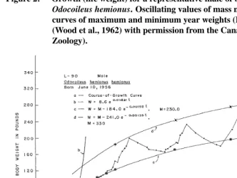
an increasing year-average weight (Wood et al., 1962). The mean yearly mass increased in males after sexual maturity throughout the period of observation (1600 days) performed on several species of deer (Wood et al., 1962). The indeterminate type of growth in male deer can be attributed to competition, here, larger mass is advantageous. This is proven by the fact that males are not allowed to actively participate in the rut until they are three or four years old. Measuring growth in deer is complicated because the typical linear measures are difficult to undertake on living animals and weight may not be a good proxy to growth. The seasonal weight changes are largely due to the accumulation and disappearance of adipose tissue and annual increment in lean body mass (assumed to be represented by the lower weight limiting curve) is relatively small after puberty is reached (Wood et al., 1962). The predicted “terminal mature weight” (the maximum asymptotic weight) is delayed or never achieved.
Figure 2: Growth (life weight) for a representative male of black-tailed deer Odocoileus hemionus. Oscillating values of mass may be limited by curves of maximum and minimum year weights (Reproduced from (Wood et al., 1962) with permission from the Canadian Journal of Zoology).
3
Mathematical description of growth
A convenient mathematical description of growth dynamics can be used to reduce the amount of measured data, explain observed patterns, compare growth rates and patterns within and between species, and to predict the future growth of these species. Two ap-proaches have been used, namely descriptive growth curves and models based on theories of growth. Often terminologically not differentiated – both are called “growth models”, the two approaches are quite different nevertheless. France and Thornley (1984) refer to these two types of description as empirical models set out principally to describe, and mechanistic models attempting to provide a description with understanding.
parameters are obtained. A wide range of questions on the growth of the organism can then be asked.
The main challenges stimulating the development of growth curves have been the de-tection of abnormal growth or disease at the early life stages in humans and the prediction and comparison of the growth of economically important animals, such as cattle, birds, and fish in order to find regimes of handling and harvesting that maximize product yield. The last problem has stimulated the development of models describing population growth, predator–prey interactions, and the coexistence of species.
A common application of growth curves in determinate growers is to establish an asymptotic size.
The great diversity of growth strategies observed in living organisms poses challenges in describing them in terms of a few simple curves. The goals of the structural approach to growth modeling are to find a suitable family of growth functions easily representing a set of longitudinal measurements, to estimate the growth parameters by fitting a function, to evaluate a goodness of fit, and to predict future growth.
Mechanistic models and theories of growth present a second, different approach – not just to fit the data but to develop a description of processes underlying growth that takes place in an organismal system. The models of growth can be simple and abstract, involving a simplistic description of build up and break-down of organism compounds and tissues, with each of these processes being related to size (model of Bertalanffy (1957)), or they may involve a detailed description of the balance of energy and compounds, the processes of consumption, an the storage and utilization of energy by different systems. Detailed models can take into account subtle processes such as changes in shape, dilution, the ratios of body reserves to somatic tissue, and the specifics of organism design and physiology, as in the Dynamic Energy Budgets theory (Kooijman, 2000).
A mechanistic model is usually derived from a differential equation relating growth rate (dy/dt) to size (y). This mathematical relationship represents the mechanism gov-erning the growth process. This approach has been extensively used for somatic growth and a large number of growth functions have been derived, such as the monomolecular, logistic, and Gompertz ones (Turner et al., 1976; France and Thornley, 1984).
The purpose of mechanistic models and theories is to understand the similarities and differences in growth in different species and to explain these differences within one mechanistic framework. Equations of growth can be derived from these models.
3.1 Typically observed patterns of growth
Several patterns are frequently observed in the growth rates of freely fed organisms. The so called exponential pattern (Figure 3, unlimited dash-dot curve) is typical for growth in certain time periods usually soon after birth.
The asymptotic growth pattern which is also called exponential (Figure 3, leveling-off dash-dot curve) applies to the length of some organisms, the size of the skull and the brain. It is characterized by a positive and steadily decreasing growth rate, therefore there is no point of inflection.
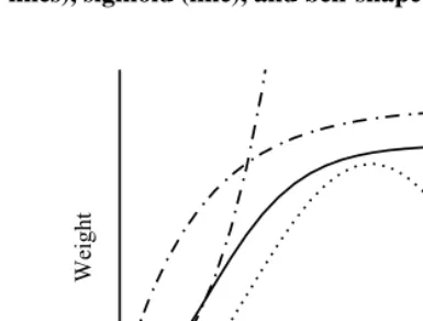
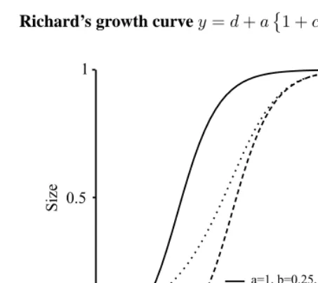
The weight and volume of the body and of most organs show a sigmoid orS-shape growth pattern (Figure 3, line). Initially, the rate of growth in mass is low but increasing. The growth rate reaches a maximum, it corresponds to the point of inflection in the curve, and then slowly declines to zero when the animals achieve their mature weight. The sigmoid curve is prevalent among determinately growing animals, and this has led to the emergence of a specific class of “sigmoid functions” describing growth. A special case of this growth mode is multiphasic growth, where several sigmoid periods follow one another throughout the development and, therefore, several growth rate maxima are present (see the human growth curve in Figure 8).
Bell-shaped growth (Figure 3, dotted curve) is observed in organs that show degener-ation and involution (thymus, bursa of Fabricius, bones in elderly humans, tree leaves at the end of the season). Organ size first increases and, after having reached a maximum, starts to decrease.
Growth can experience complex patterns, such as non-monotonic, oscillating changes in mass (e.g. in animals with strong seasonal differences in the quality of feed), and in perennial plants. Often, it is difficult to separate growth from the accumulation of resources when change in mass is the summary measure of these effects. As an example, the cyclic changes of mass due to the accumulation and utilization of fat in deer are overlayed on the monotonic growth of fat-free mass (see Figure 2). The growth pattern observed depends on the measure of growth selected – even in isomorphs the curves of growth in linear size and mass or volume will have different shapes.
For these patterns of growth, a multitude of growth curves has been proposed. None of them, however, meet the demands of a biophysical model in its narrow sense. Therefore, growth curve analysis is more or less a phenomenological analysis of growth courses.
3.2 Growth curves as empirical models
Figure 3: Frequently observed growth patterns: “exponential” (both dash-dot lines), sigmoid (line), and bell-shaped (dotted line).
Age
Weight
and cattle, which have been of primary interest. Since determinate growth is character-ized by a maximum size that is approached with a diminishing growth rate, such curves are also called asymptotic. Examples are the exponential (with the declining growth rate), logistic, Richards, Gompertz, von Bertalanffy curves. All these curves except for the ex-ponential have sigmoidal shape. In all following equations,twill denote the age of the individual, andy=y(t)– its size.
3.2.1 Curves for determinate growth
The exponential growth curve
Assume that the rate of growth is proportional to the size: dy/dt=by. The solution of this differential equation defines the exponential growth curve
y=y0ebt. (1)
Parametery0is the initial size (at age zero). Forb > 0, this function will usually only be applicable to temporarily limited periods of growth (e.g. at the early growth stage) (see also the logistic growth curve (Figure 4)). Forb <0, this may be a good model of exponential decline, e.g. of some decaying activity.
time and size scales, we obtain a variant of the exponential growth curve which allows for an asymptotic approach to the maximum sizey∞:
˜
y=y∞(1−e−bτ), (2)
This form of curve is often referred to as the von Bertalanffy curve, but note that the actual solution (20) for the von Bertalanffy model (19) has the form of an exponential function (1) raised to the power1/(1−m). For animals, typically2/3< m <1so1/(1−m)>3. Equation (2) can also be written in the form of y = y∞(1−e−k(t−t0)), where t
0 is
the theoretical age at which the organism would have zero size. kis often called the Brody growth coefficient, or the rate at whichy∞is achieved or a measure of the rate at which the growth rate declines. Brody himself used this type of “inverted” exponential growth function in the second part of his sigmoidal functions (6, 7). Generally, a highkis associated with fast early growth, low age and size at maturity, high reproductive output, a short life span, and a short max length. The exponential curve of this form is a particular case of monomolecular growth, in which the rapid initial growth is followed by a leveling off.
The exponential curve can be applied to mass as well as to length. It fits length better than mass and works better for older ages. During larval and early juveniles stages, a sigmoid curve is more applicable.
Monomolecular growth
One of the simplest assumptions leading to a growth curve approaching a limiting value
y∞is that the growth rate is proportional to the difference between the level and the actual size, i.e. dy/dt=b(y∞−y), whereb >0. The solution to this differential equation is the monomolecular growth function:
y=y∞−(y∞−y0)e−bt=y∞−δe−bt, (3)
Here,y0 is the initial size and ify0 = 0, the solution reduces toy = y∞(1−e−bt), a special case (2) of exponential growth curve. The monomolecular curve has rapid initial growth followed by a leveling off.
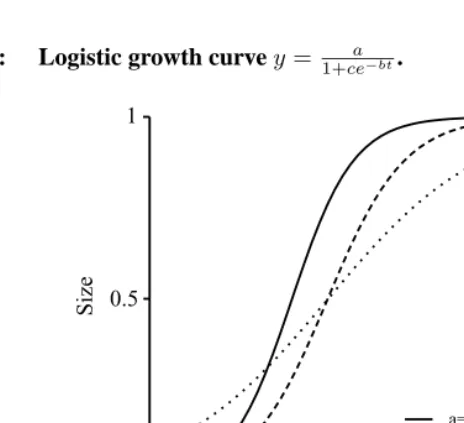
Logistic growth
The solution of this differential equation is exponential growth (1). Growth at the second stage is linear in time, i.e. y = y0+bt. The third stage is a limiting stage, where the growth rate approaches zero and the weight approaches a limiting levely∞. The fourth stage will not be considered here. By considering the first three stages only, the growth can be described by a differential equation: dy/dt= by(y∞−y)/y∞. The solution to this is known as the logistic curve
y= 1 +y∞
eη−bt. (4)
The size, y, approaches the upper limity∞ as time tends to infinity. The parameterη
has no direct interpretation but may be seen as a measure of the difference in weight from birth to maturity since isolatingη at timet = 0and lettingα = y0 we find that
η= ln(η/α−1). Inserting this result into the equation of the logistic curve (4), we can write the following re-parameterized version:
y= αy∞
α+ (y∞−α)e−bt. (5)
This way of expressing the logistic curve has the advantage that the initial weight is a parameter in the model. The logistic curve (Figure 4) is sigmoid, has a lower limit at0, and an upper limit aty∞. The curve is symmetric around the point of inflexiony=y∞/2
where the absolute growth rate is maximal. The last property is one of the drawbacks of the logistic growth curve. The Gompertz growth curve is more flexible.
The Sigmoid (Brody) curves
As mentioned, sigmoid patterns of growth are frequently observed in animals that are determinate-growers. Brody (1945) suggested growth be expressed by a continuous curve with a discontinuous slope at the inflection point – the sigmoidal curve, often referenced to as Brody’s curve. He described growth as “self accelerating” before and “self inhibiting or decelerating” after aget, and suggested the following mathematical description:
y=y0ebt,0≤t≤t, (6)
y=y∞
1−e−k(t−t∗)
, t≤t (7)
Here,y0is the initial live weight of the animal (i.e. the weight at birth),bis the exponential growth constant in the growth acceleration phase,y∞denotes the mature live weight,k
Figure 4: Logistic growth curvey= a
1+ce−bt.
0 20 40 60
0 0.5 1
Age
Size
a=1, b=0.25, c=100 a=1, b=0.2, c=100 a=1, b=0.1, c=10
growth data for many animals very well. This motivated Brody to call the parametersy∞,
k, andt∗genetic “constants”, and to create an extensive table listing the values (Brody, 1945; Parks, 1982).
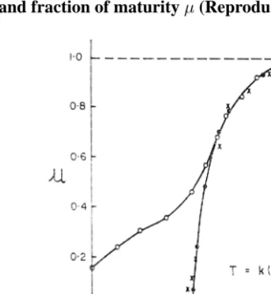
Brody suggested to express growth in coordinates of the degree of maturity (µ = y/y∞) versus normalized ageT, using transformationsT =k(t−t∗)andu= 1−e−T,
0< T, and demonstrated that the growth data for a wide range of animals lie on the same graph (Figure 5). The coincidence of the growth data from such widely differing species forT >0is remarkable. A plot in these coordinates shows where the determinate growth of different animals has the same features and where it differs (Parks, 1982).
The Richards curve
Richards (1959) was the first to apply to the plant sciences a growth equation developed by von Bertalanffy to describe the growth of animals (France and Thornley, 1984). The Richards curve is very general and has the monomolecular (ν =−1), the logistic (ν = 1), and the Gompertz (ν = 0) curves as special cases, whereν is a parameter in Richard’s equation. As with the other growth curves, there are various ways of writing the curve equation. One of them (Labouriau et al., 2000) is:
y=α{1 +sign(ν)eβ−κt}−1/ν. (8)
Figure 5: Growth in rats, cows and man expressed in Brody’s normalized ageT
and fraction of maturityµ(Reproduced from Parks (1982)).
signis a signum function (sign(x) = −1, x < 0, 0,x= 0and 1,x > 0). The curve has an inflection point at the time pointt= (β−ln(|ν|)/κ. The expected response at the inflection point is given byµ=α(ν+ 1)−1/ν.
The point of inflection now is able to occur at any fraction of the final weight, asν
varies over range−1≤ν <∞. Parameterκcontrols the position of the inflection point. The intercept (the value at t=0) of the Richards curve is
y0=α1 +sign(ν)eβ−1/ν. (9)
Parameterαis the limiting size (the asymptote of the curve). Parameterνdetermines the relative value (compared to the limiting size) of the Richards function at the inflection point:
y
α = (ν+ 1)
−1/ν. (10)
Figure 6: Richard’s growth curvey=d+a1 +ce−b(t−m)−1/c .
0 20 40 60
0 0.5 1
Age
Size
a=1, b=0.25, c=0.5, d=0, m=15 a=1, b=0.25, c=0.5, d=0, m=25 a=1, b=0.25, c=2, d=0, m=25
dthe lower asymptotic size, b denotes the average growth rate, m the age of maxi-mum growth, cdetermines whether max growth occurs early or late, andy = α{1− β1e−β2t}β3. In practice, the Richards curve is rather difficult to fit due to numerical prob-lems. The model has too many parameters for practical situations and is an example of over-parametrization.
The Gompertz growth curve
The Gompertz equation arises from models of self-limited growth where the rate de-creases exponentially with time. The model was first introduced to describe growth in the number of tumor cells which usually follows a sigmoidal growth pattern. The equation is a solution of the differential equation:
dN
dt =λNln(θ/N); N(0) =N0, (11)
whereN is the number of tumor cells at timet.
Let the growth rate be expressed by the differential equationdy/dt=kye−bt, where
bandkare constants. The solution is
wherey∞ is the asymptotic size. Alternatively, the growth rate may be defined by a differential equation of the formdy/dt = y(β −αlny), whereαandβ are constants. The solution of this equation is:
y=eC1(e−α(t+C2)+β)/α
(13)
Figure 7: The Gompertz growth curvey=ae−ce−bt.
0 20 40 60
0 0.5
1
Age
Size
a=1, b=0.25, c=100 a=1, b=0.2, c=100 a=1, b=0.1, c=10
Solutions of these models are know as the Gompertz growth curve, which is usually expressed in the form
y =y∞e−ce−bt, (14)
wherey∞ > 0 is the final (asymptotic) size, parameter b > 0 describes the decay in the specific growth rate, and parameterc > 0controls the difference between the initial and final weight. The point of inflection is the time point wherey = y∞/e, this gives
known as the log-log link function: ln(−ln(y/y∞)) = lnc−bt.Asymmetry can be in-verted by applying an exponent to both parts:y=y∞(1−e−ce−bt),this is known as the complementary Gompertz curve. Again, the initial values can be found by a transforma-tion known as the C-log-log link functransforma-tion:ln(−ln(1−y/y∞)) = lnc−bt.
The Gompertz growth model should not be confused with the Gompertz model of mortality,µ(t) =aebt, introduced by Gompertz (1825) to describe increase of mortality,
µ, in adult humans with age. It is well known in mathematical demography.
The von Bertalanffy curve
Bertalanffy (1941) proposed the first model of animal growth based on metabolic pro-cesses (20). It will be discussed in section 3.3.1. The solution of this model, and more generally, asymptotic growth curves of the form
y=y∞−(y∞−y0)e−ct (15)
are referred to as the “von Bertalnaffy” growth curves and widely used to describe growth in animals and humans. This is a case of asymptotic growth from initial sizey0to asymp-totic sizey∞with a decreasing rate. The curve has no inflection point.
3.2.2 A curve for indeterminate growth
Curves with upper limits cannot be used to describe indeterminate growth. The exponen-tial growth curve increasing monotonously is too rough to use. Tanaka (1982) introduced a four-parameter curve for indeterminate growth that has an initial period of exponential growth followed by an indefinite period of slow growth. It was the first model that rea-sonably described indeterminate growth. The function, which he named ALOG, has the form:
y=√1 f ln
2f(t−c) + 2f2(t−c)2+f a
+d, (16)
wherea >0, c , d > 0,andf >0are parameters. The curve monotonously approaches infinity astincreases. The growth rate isdy/dt= 1/f(t−c)2+a. It is positive over all range and reaches a maximum att = c (the inflection point), therefore the growth curve has a sigmoid shape nearc. The growth curve was first applied to data on spoon shell Laternula anatina and Theora lubrica (Tanaka and Kikuchi, 1979, 1980).
3.2.3 Multiphasic growth curves
best by a combination of separate growth curves for each period. Koops (1986) pro-posed to use a multiphasic growth curve formed as a summation of several (n) logistic growth functions. Human height growth curves of this type are known as “double lo-gistic” (n = 2) and “triple logistic” (n = 3) growth curves (Bock and Thissen, 1976). He noted that there is evidence for the existence of growth phases in the weight growth curves of animals. The fit of the multiphasic growth curve, applied to pika, mice, and rabbit weights, was shown to be superior to the monophasic model in terms of residual variances and the absence of the autocorrelation of residuals.
3.2.4 Polynomial growth curves
The use of polynomials to represent growth curves has been accorded high importance by many researchers (Goldstein, 1979; Wishart, 1938) since polynomials can approximate any curve. In this sense, polynomial curves have certain advantages over other types of curves. Polynomials are simpler to fit, and it is also easier to work out the statistical distribution properties of the parameters when fitted to a sample of individuals than in the case of curves such as the logistic one (Goldstein, 1979). Sandland and McGilchrist (1979) described and fitted the third degree polynomial model using a stochastic approach to the preadolescent human height data.
Yi and Li-feng (1998) introduced a model based on the Gompertz and polynomial model:
y=ceni=0−1αiti. (17)
Hasani et al. (2003) introduced a type of polynomial model of ordernto fit growth data during infancy:
y=α0+
n
k=1
{(−1)k+1α k
tk
ck}, (18)
They described how to select the order of the model and used the model of order 6 to fit the data set on US children.
For a mathematical entrance to the subject of growth curves, refer to (France and Thornley, 1984, ch. 5). Moreover, (Draper and Smith, 1981, ch. 10), (Mead et al., 1993, ch. 12), and many other textbooks consider growth curves.
3.2.5 A description of human growth
intervals, usually early childhood, several curves have been proposed. The model of von Bertalanffy (see 3.3.1) is widely used to describe growth in animals and humans. Jenss and Bayley (1937) suggested one of the early curves of human growth in height during childhood in the form ofy = a+bt−ec−dt. The curve is a combination of the von Bertalanffy’s growth curve and the linear growth curve. Count (1943) introduced a curve for growth patterns in human height in the form of y = a+bt+clog(t). Jolicoeur (1963) introduced a multivariate allometry model. Krüger (1965) proposed the so-called Reziprok function. Tanaka (1976) suggested the double exponential curve. Bock and Thissen (1976) introduced a triple logistic model to describe human growth in height to adulthood. Thissen et al. (1976) proposed a two-component model for individual growth and tested the model by comparing the patterns of growth in the stature of subjects from the four major U.S. longitudinal growth studies. He described problems comparing data from independent growth studies and offered solutions. Preece and Baines (1978) intro-duced a new family of mathematical functions to fit longitudinal growth data. All mem-bers derive from the differential equationdh/dt =s(t)(h1−h), whereh1is the adult size ands(t)is a function of time. The form ofs(t)is given by one of many functions, all solutions of differential equations, thus generating a family of different models. Shohoji and Sasaki (1987) modified and extended Count’s model toy =a+bt+clog(1 +dt). In 1989 Nelder introduced a modified logistic model and Jolicoeur and Pontier (1989) introduced a generalization of the logistic model. An asymptotic lifetime growth model of height was introduced by Kanefuji and Shohoji (1990) by modifying a fundamental growth model considering a relative measure of maturity. This model, compared to the previous model of Preece and Baines (1978) and the (Jolicoeur et al., 1991, 1992) (JPA1), was the best considering the goodness of fit. Jolicoeur et al. (1992) proposed an improved version of the JPA1 model which is a modified version of the JPA1 model and the triple logistic model of Bock and Thissen (1976). The new model is called the JPA2 model.
The curves most commonly used today in studies on humans growth and develop-ment are the Gompertz model, the triple logistic model of Bock and Thissen (1976), the modified logistic model of McCullagh and Nelder (1989), a generalization of the logistic model by Jolicoeur and Pontier (1989), the Preece and Baines (1978) model, the modified version of the Shohoji and Sasaki (1987), the model of Kanefuji and Shohoji (1990), JPA1 (Jolicoeur et al., 1991, 1992), the model of Jolicoeur et al. (1988) for human growth in childhood, the latter which is widely used and referenced to as JPPS, and especially JPA2 models.
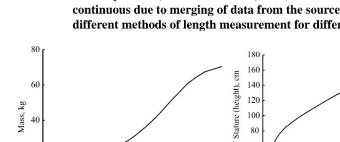
Figure 8: Human growth. a) body mass from conception to the age of 20; b) length of foetus from conception to birth / mean length of a baby (0 – 2 years) / stature of boys (2 – 20 years); birth occurs at aget= 0. Data on foetus development for USA children from (MedlinePlus Medical Encyclopedia, 2006; Moore and Persaud, 1998), post-birth data for USA boys from (Kuczmarski et al., 2000). The curves are not continuous due to merging of data from the sources and the use of different methods of length measurement for different ages.
0 5 10 15 20
0 20 40 60 80
Age, years
Mass, kg
-1 0 0 5 10 15 20
20 40 60 80 100 120 140 160 180
Age, years
Length / Stature (height), cm
-1
by separate curves with different parameters (see 3.2.3), and finally to polynomial curves (see 3.2.4).
Recent studies have found a positive relationship between stature and reproductive success of men in contemporary populations (Pawlowski et al., 2000; Mueller and Mazur, 2001; Nettle, 2002a). This appears to be due to their greater ability to attract mates. The study of Nettle (2002b) examine the life histories of a British women and found height to be weakly but significantly related to reproductive success. The relationship was U-shaped. This pattern was largely due to poor health among extremely tall and extremely short women.
men in populations with polygynous marriage because of intra-male competition for fe-males, and interaction between female size and probability of birth-related complications (Rogers and Mukherjee, 1992; Guégan et al., 2000). Male and female weights are tightly correlated and dimorphism is not a simple allometric function of size. Lindenfors and Tullberg (1998) studied the relationship between primate mating system, size and size dimorphism.
3.2.6 A description of cattle growth
The description of growth in cattle has a purpose similar to that in humans – detecting early deviations in development, future growth, and the projection of the final size of the animal. Several classical equations have often been used to describe growth patterns and predict growth in cattle, and several new ones have been specifically developed: the Gompertz equation (mass) and the logistic (mass), the Brody, the von Bertalanfy (length), Feller, Weiss and Kavanau, Fitzhugh, Richards (variable), Laird, and Parks equations, and the Tanaka equation (though it was created for indeterminate growth). Summarized de-scriptions can be found in (Arango and Van Vleck, 2002; Parks, 1982). See also (Brown et al., 1976; Fitzhugh Jr., 1976; Johnson et al., 1990). Parks (1982) covered various as-pects of describing cattle growth and proposed his own synthetic growth model. Recently, another model of cattle growth was proposed by (Hoch and Agabriel, 2004a,b).
3.3 Theories and mechanistic models of growth
3.3.1 A model of von Bertalanffy
Table 2: Metabolic types and growth types. Growth is measured as increase in linear size. Modified from (Bertalanffy, 1951).
Metabolic type Growth type Examples I. Respiration
surface-proportional
(a)Linear growth curve: attaining
without inflexion a steady state.
(b) Weight growth curve: sigmoid, attaining, with inflexion at c. 1/3 of final weight, a steady state
Lamellibranchs, fish, mammals (disputed; true at least in rats), certain invertebrates (isopod crustaceans, mussels, Ascaris)
II. Respiration weight-proportional
Linear and weight growth curves
exponential, no steady state
at-tained, but growth intercepted by metamorphosis or seasonal cy-cles
Insect larvae, Orthoptera,
Heli-cidae land snails, hemimetabolic
insects, Annelids (e.g. earth worms)
III. Respiration inter-mediate between sur-face and weight pro-portionality
(a) Linear growth curve: attaining
with inflexion a steady state.
(b) Weight growth curve: sigmoid, similar to I(b)
Planorbidae (pond snails), Lim-naea, Planarians
Bertalanffy (1941, 1942) proposed the first model of animal growth based on metabolic processes and Pütter’s idea of balance between the processes of catabolism and anabolism in the form
dM/dt=ηMm−κMn, (19)
where changes in body mass,Mare given as difference between the processes of building up and breaking down;ηandκare constants of anabolism and catabolism respectively, and the exponentsmandnindicate that the latter is proportional to some power of the body mass. The solution of the differential equation (19) (forn= 1) is
W ={η/κ−[η/κ−W0(1−m)]e−(1−m)κt}1−1m, (20)
whereW0is the weight at timet= 0(Bertalanffy, 1957). This growth curve is frequently used to describe animal growth and referred to as the “von Bertalanffy” of “Brody– Bertalanffy” growth curve because it resembles the inverted exponential growth function used by Brody in his sigmoidal function. It is the first growth curve specially designed to describe an individual. The curve has been proposed for animals, but is widely used for humans, too.
3.3.2 The theory of growth of Turner et al.
There have been many contributors to kinetic theories of growth, such as Verhulst (1838), Pearl and Reead (1920), Medawar (1940), Bertalanffy (1941), Lotka (1956), Bertalanffy (1957), Richards (1959), Nelder (1961), Quetelet (1968) and Turner et al. (1969). The early history of the subject was reviewed by Glass (1967).
Turner et al. (1976) presented a generalized theory of growth based on three postu-lates. The first asserts that the rate of growth is jointly proportional to the monotonic function of the generalized distance from the initial size to the present size (“reproductive capability”), and to a monotonic function of the generalized distance from the present size to the ultimate size (“the limiting factor”). The second postulate restricts the monotonic function to power (or “mass action”) functions. The third postulate constrains the model to a mathematically tractable set that nevertheless is sufficiently general to include the Malthusian, Gompertz, logistic, and con Bertalanffy-Richards growth models.
On the basis of these postulates they obtained a generic growth function that has as special limiting cases several well-known growth curves such as the Verhulst logistic curve, the Gompertz curve, and the generalized growth curve of von Bertalanffy and Richards. In addition, they obtained several new forms. The relation between their growth curve and other well-known growth curves is shown in Figure 9. The most general case is termed by Turner et al. (1976) the “generic growth model”. Other special cases are termed “hyperGompertzian” and “hyperlogistic growth”.
3.3.3 Park’s theory of animal feeding and growth
Parks (1982) analyzed a large number of sets of experimental growth and feeding data for cattle and domestic animals on various diets and under various feeding regimes, and looked for deterministic elements in animal feeding and growth patterns that could form the basis of a testable theory. He integrated these studies into a mathematical theory of feeding and growth, allowing to predict animal growth under different feeding regimes. The theory is related to the laws of energy balance. Parks’ theory is sufficiently robust to be used in studies on the diet and nutrition of other growing animals. He illustrated the applicability of his theory in a long-term experiment on two genotypes of chicken and discussed the implications of the theory in genetic experimental work on bending the growth curves of mice and chicken by selection techniques and in the economics of intensive animal productions.
3.3.4 The theory of Dynamic Energy Budgets of Kooijman et al.
Figure 9: The interrelation between the growth curve of Turner et al. (1976) and other well-known growth curves (Reprinted from Math. Biosci. 29, Turner, M., E. Bradley, K. Kirk, and K. Pruitt A theory of growth pp. 367-373, Copyright 1976, with permission from Elsevier).
are feeding, digestion, storage, maintenance, growth, development, reproduction, product formation, respiration, and aging. The theory amounts to a set of simple mechanistically inspired rules for the uptake and use of substrates (food, nutrients, light) by individuals. It has far-reaching implications for population dynamics and metabolic organization. The theory explains the dynamics of only one variable, size (i.e. growth).
that the von Bertalanffy growth rate is (approximately) inversely proportional to the maxi-mum volumetric length. This is shown for data on 261 widely different species. The DEB theory results in some well known empirical models for special cases and, therefore, has considerable empirical support.
3.3.5 The general model of ontogenetic growth of West et al.
West et al. (2001) proposed a general quantitative model based on fundamental principles for the allocation of metabolic energy between the maintenance of existing tissue and the production of new biomass. They derive the values of the parameters governing growth from basic cellular properties and construct a single parameterless universal curve that describes the growth of many diverse species (Figure 10). The model provides the basis for deriving allometric relationships for growth rates and the timing of life history events (Charnov, 1993; Peters, 1983; Calder III, 1984).
3.4 Selecting the growth model
Many growth curves have been proposed to describe growth in humans and animals. Some curves were proposed specifically to fit human data and cattle data. Most curves and models of growth describe linear growth (in length or height), other better fit the dynamics of mass.
Growth functions have certain mathematical limitations that need to be considered when choosing an appropriate model. For example, if a function does not have a point of inflection, the result of fitting will yield none even if the data show it.
Some functions were constructed to describe a specific stage of growth. For example, many functions proposed for a specific interval of rapid growth (infancy) in humans are unlimited and cannot be applied to the whole life period of the determinate grower.
A specific growth curve is sometimes chosen by simply looking at the plots of the data. Sometimes it is preferable to select or construct a function that has a biological in-terpretation and meaningful parameters. The functional relationship in the growth models is often derived from knowledge on the rates of growthdy/dttypically as a solution of a differential equation.
Figure 10: Universal growth curve. A plot of the dimensionless mass ratio,
r= 1−R≡(m/M)1/4, versus the dimensionless time variable,
t= (at/4M1/4)−ln[1−(m
0/M)1/4], for a wide variety of
determinate and indeterminate species. When plotted in this way, the model of West et al. (2001) predicts that growth curves for all
organisms fall on the same universal parameterless curve1−e−t (shown as a solid line). The model identifiesras the proportion of total lifetime metabolic power used for maintenance and other activities (Reproduced by permission from Macmillan Publishers Ltd: Nature West, G. B., J. H. Brown, and B. J. Enquist (2001). A general model for ontogenetic growth [Letters to Nature]. Nature 413, 628-631, copyright 2001).
0 0.25 0.50 0.75 1.00 1.25
Dimensionless mass ratio, r
Dimensionless time, t
Pig Shrew Rabbit Cod Rat Guinea pig Shrimp Salmon Guppy Hen Robin Heron
Cow
The process of constructing growth curves is an ongoing process driven by the aim to create a parametric function (producing a family of growth curves) with a minimum number of parameters and the best fit to the growth data of a given organism and growth period. When several models are being compared the quality of fit is considered in the sense of some criteria, such as the Akaike Information Criteria (AIC) (Akaike, 1972) which allows to account for a different number of fitted parameters.
Data for determinate growth in length (or mass1/3) often is well fitted by the von Bertalanffy growth curve (Kooijman, 2000). The most frequently used growth curves also include the Gompertz and sigmoidal logistic curves (Tanaka, 1982). The exponential growth curve (Brody, 1945), the Reziprok function (Krüger, 1965), and the double ex-ponential curve (Tanaka, 1976) also have been used sometimes as growth curve. Except for the exponential curve, these curves increase monotonically with age and converge to a finite value.
Zullinger et al. (1984) tested the fit of the von Bertalanffy, Gompertz, and logistic sigmoidal growth curves to data on the maximum of 331 mammal species in 19 orders; most data was obtained from longitudinal studies on captive animals. The best fit on a sample of 49 species was provided by the von Bertalanffy and Gompertz equations. The authors discuss the problems of fitting mammalian growth data and list the parameters of the Gompertz growth function for data from 331 species. They also provide references to the original data. Heppell et al. (2000) gives a list of available life tables for 50 mammal populations. More information on growth in mammals can be obtained from (Vaughan et al., 2000).
4
A comparison of growth between species
4.1 Allometry and scaling relationships
The relationship of body size to the anatomical, physiological, behavioral, and ecological characteristics has since long been a focus of interest in zoology. As one considers animal species of different size, regular and predictable changes are seen in the relative propor-tions of the organs and the relative rates of physiological processes such as the metabolism and growth (Damuth, 2001). These scaling relationships are called allometries and have many ecological and adaptive implications (Kleiber, 1975; Schmidt-Nielsen, 1984; Pe-ters, 1983). The following allometric expressing the scaling of some physiological or morphological parameter,yin accordance with changes in body size,Mis well known:
y=aMb. (21)
The search for similarities in the metabolic organization and growth of animals re-ceived much attention, one of the directions is looking for different invariants. Brown and West (2000) discussed diverse questions and aspects of scaling in animals and plants. Charnov et al. (2001) reported that a prominent feature of comparative life histories in fish and other indeterminate growers is the approximate invariance across species of dimen-sionless numbers made up from reproductive and timing variables. The two best known are age at maturity divided by average adult lifespan, and the proportion of body mass given to reproduction per year multiplied by the average adult lifespan.
Invariants have been empirically observed in animals also on the population level: species differing in body mass,M, by many orders of magnitude tend to have almost equal rates of energy use per unit area by the population, because of an inverse allometric scaling relationship between energy use by the individual, or its metabolic rate,B, and the maximal population density,Nmax. BecauseB ∝ M3/4andN
max ∝M−3/4, energy use is proportional toBNmax∝M3/4M−3/4∝M0. This phenomenon was defined by
Damuth (1981) as “energy equivalence”. Enquist et al. (1998) showed that this also holds for plants, namely that the allometric scaling of bothBandNmaxappears to be the same as in animals.
Growth rates, or rates of production of new biomass, are of fundamental importance in linking physiological processes to adaptively important features, such as reproductive rates and other life history variables. Among animal species, the rates of biomass produc-tion and growth are proporproduc-tional to the metabolic rate, which scales as the 3/4 power of body mass (Kleiber, 1975; Peters, 1983).
mitochondria, and oxidase molecules. They hypothesize that natural selection tends to maximize both metabolic capacity, by maximizing the scaling of exchange surface ar-eas, and internal efficiency, by minimizing the scaling of transport distances and times. These design principles are independent of detailed dynamics and explicit models and should apply to virtually all organisms. Other researchers doubt the applicability of the “3/4 rule” of energy–size relationship. Dodds and Rothman (2001) considered value 2/3 obtained from simple dimensional relationships to be a null hypothesis testable by empir-ical studies. They re-analyzed several data sets for mammals and birds and found little evidence for rejecting b = 2/3 in favor ofb = 3/4. The authors argued that present theories forb= 3/4require assumptions that render them unconvincing for rejecting the null hypothesis thatb = 2/3. The value of the scaling exponent,b, is a point of active debate in the literature, with sound arguments for and against geometric (b = 2/3) and quarter-power (b= 3/4) scaling.
4.2 Animal-plant unification
Plants exhibit degrees of modular construction, indeterminate growth, and form varieties that are greater than those shown by animals. However, until recently, the scaling of basic processes such as the metabolism and growth had remained undocumented for a representative sample of plant species. A book by Niklas (1994) on plant allometry is an early attempt to provide a unified treatment of plant form and function from an allomet-ric perspective. Niklas (1994); Niklas and Enquist (2001) discussed allometry in plants and presented empirical allometric scaling relationships for rates of annual plant biomass production (“growth”), different measures of body size (dry weight and length) and pho-tosynthetic biomass (or pigment concentration) per plant (or cell) in species ranging from unicellular algae to large trees. Annualized rates of growthGscale as the3/4power of body massM over 20 orders of magnitude ofM (i.e. G ∝ M3/4); plant body length
These new analyses reveal that growth scales among plants in the same way as it does among animals, and support the growing realization that the same scaling rules may apply to both animals and plants for similar reasons (Damuth, 2001). Many attempts have been made to consider scaling rules in plants and animals and to create a unifying approach, explaining the similarities between the structural and metabolic organization. Damuth (2001, 1998) reviewed advances in the comparative growth allometry of plants and animals and research towards unifying common laws of scaling and discussed general models that can be applied (with different assumptions) to both animals and plants noting among them the work of Banavar et al. (1999) on transportation networks and the theory of dynamic energy budgets (Kooijman, 2000). He reviewed the study of Niklas and En-quist (2001) on plant allometry and compared the results obtained on plants (trees) with those for “warm-blooded” (endothermic) and ”cold-blooded” (ectothermic) metabolic an-imals. He compared the rates of growth of animals and plants over the size ranges that they have in common (Figure 11). The realized somatic growth rates of both plants and animals of comparable body mass are remarkably similar. This suggests that the cells of both plants and animals are similarly limited in the rates by which they can effectuate growth, just as the abilities of different-sized plants and animals to deliver energy to their cells are similarly constrained by scaling relationships. Banavar et al. (2002) proposed a set of scaling relations for age, mass, and other physiological traits that allow to display ontogenetic changes in different organisms (showing determinate growth) on a universal growth curve with dimensionless time and a mass ratio.
West et al. (2002) described the allometric scaling of the metabolic rate on a large scale, from molecules and mitochondria to cells and mammals. They performed a new analysis of the allometry of mammalian basal metabolic rate that accounts for variation associated with body temperature, digestive state, and phylogeny using data encompass-ing five orders of magnitude variation inM and featuring 619 species from 19 orders. The authors found no support for a metabolic scaling exponent of3/4. Their results demonstrate thatB∝M2/3(White and Seymour, 2003).
4.3 Growth and conservation laws