R E S E A R C H A R T I C L E
Open Access
An evaluation of computerized adaptive
testing for general psychological distress:
combining GHQ-12 and Affectometer-2 in
an item bank for public mental health
research
Jan Stochl
1,2,3*, Jan R. Böhnke
1,4, Kate E. Pickett
1and Tim J. Croudace
1,4,5Abstract
Background:Recent developments in psychometric modeling and technology allow pooling well-validated items
from existing instruments into larger item banks and their deployment through methods of computerized adaptive testing (CAT). Use of item response theory-based bifactor methods and integrative data analysis overcomes barriers in cross-instrument comparison. This paper presents the joint calibration of an item bank for researchers keen to investigate population variations in general psychological distress (GPD).
Methods:Multidimensional item response theory was used on existing health survey data from the Scottish Health
Education Population Survey (n= 766) to calibrate an item bank consisting of pooled items from the short common mental disorder screen (GHQ-12) and the Affectometer-2 (a measure of“general happiness”). Computer simulation was used to evaluate usefulness and efficacy of its adaptive administration.
Results:A bifactor model capturing variation across a continuum of population distress (while controlling for artefacts due to item wording) was supported. The numbers of items for different required reliabilities in adaptive administration demonstrated promising efficacy of the proposed item bank.
Conclusions:Psychometric modeling of the common dimension captured by more than one instrument offers the
potential of adaptive testing for GPD using individually sequenced combinations of existing survey items. The potential for linking other item sets with alternative candidate measures of positive mental health is discussed since an optimal item bank may require even more items than these.
Keywords:Computerized adaptive testing, General Health Questionnaire, Affectometer, Item Response Theory
Background
Assessment of the psychological component of health via rating scales and questionnaires has a long and continuing history. This is exemplified by the work of Goldberg on his General Health Questionnaire (GHQ) item set(s) [1], but also by many others who have worked on question-naires measuring “general health” [2]. Goldberg’s GHQ
instruments are intended to be scored and used as an as-sessment of risk for common mental disorder(s) and have become established in health care, help seeking and epi-demiological studies including national and cross-national surveys. However, there have also been new and influ-ential measures developed for application in this set-ting, introduced by researchers from the fields of health promotion, positive psychology, and public (mental) health. Consequently, over the past two decades it has be-come increasingly common for national and international research studies and health surveys to broaden measure-ment to a wider range of psychological health concepts in * Correspondence:[email protected]
1Department of Health Sciences, University of York, York, UK
2Department of Psychiatry, University of Cambridge, Cambridge Biomedical
Campus, Box 189, Cambridge CB2 0QQ, UK
Full list of author information is available at the end of the article
populations [3]. This has resulted in multi-faceted defini-tions and new instrument convendefini-tions for fieldwork [4] such that more than one instrument is now likely to be included in health or well-being surveys.
Presently, a number of alternative instruments appear popular. Hence there are choices and opportunities for researchers and survey designers to experiment with dif-ferent assemblies, subsets and orderings of existing items within and across instruments [5–7]. Our impression is that this has been rare to date and therefore several instruments that may all assess a common construct may exist and have been developed in parallel [8]. If this argument holds, then there may be no need to invent or introduce new items or instruments, as existing item sets might be sufficient or adequate, and already complement each other in this regard. If this is the case, they can be combined in order to achieve accurate and efficient meas-urement of population level variation in public health research.
We suggest that, over the past decade, too much of the debate about the measurement of well-being has been about specific instruments, i.e. fixed collections of items, not about the items themselves. Instead of looking at whole instruments and correlations between their scores in order to try to gauge their similarity, the use of item response theory (IRT) based models and joint ana-lysis of items (“co-callibration”) [8–10] may be of greater value in advancing understanding and measurement of psychological distress variation (and dimensions). Such activities make it possible to identify useful items, the extent of overlap between instruments and optimal item sets for specific assessment purposes. Even more than that, IRT models can help to support those who might wish to administer assessments in a shorter time, they offer potentially higher face validity for the individual re-spondents, yet still with a level of precision that is high enough for any given scientific or practical purpose, as be-fits any particular study or set of surveys. This can be achieved by employing computer-adaptive procedures that do not require researchers to depend on any single specific instrument or measure, but rather to use a broader“pool” of content consisting of a large collection of items cali-brated using IRT: a practice that has become known as computerized adaptive testing (CAT) [11]. Since there is potential for most modern surveys to use technologies that allow items to be administered via apps, on mobile devices or through conventional or cloud-based computing plat-forms, there is no reason why this technology should not be used to its maximum potential, to support adaptive test-ing ideas in the field of survey research.
In this paper we present such a joint analysis. Our aim is to combine item sets from two instruments (the GHQ-12 and Affectometer-2) and to offer them as an item bank for general psychological distress [12] measurement. The main
aim of such an analysis is the quantification of similarities and overlap across all items - as well as their item parame-ters - that can be used for further implementation as an
“item bank”. Since we will invoke psychometric principles and models that allow for adaptive measurement, we will also emphasize how the measurement error considered under this approach can enhance narratives about lowest permissible measurement precision across individuals.
To this end, we first compared plausible structural models that were derived from the literature for each in-strument and then fit an appropriate latent variable model (from the family of IRT models). This approach allowed us to map GHQ-12 and Affectometer-2 items onto a com-mon dimension measured by both instruments. Hence this general psychological distress "factor" (dimension) was de-fined via bifactor modeling [13]. Based on this model we next assessed inter-item dependencies and the position of the item parameters on the latent continuum to identify which items of the two instruments were possibly ex-changeable [14] and would align to one metric.
Building on the previous steps, we then explored the feasibility of administering the joint item-set as a comput-erized adaptive test drawing on the 52-item bank. In the simulation study we took an additional opportunity to compare different estimation procedures and configura-tions of the CAT algorithms as well as exploring the num-ber of items that are necessary to reliably assess a general psychological distress factor. In doing so we aimed to meet the measurement and practical needs of public mental health researchers.
Methods
Multi-item questionnaires to be jointly calibrated: integrative data analysis approach
Two instruments are introduced as key measures in the dataset chosen for our analysis. We chose instruments for which there is either extensive literature, or interest-ing items: the former is our justification for usinterest-ing GHQ-12, and the latter for including Affectometer-2.
The Affectometer-2 is a 40-item scale developed in New Zealand to measuregeneral happinessas a sense of well-being based on assessing the balance of positive and negative feelings in recent experience [16]. Its items con-tain both simple adjectives and phrases. The Affectometer-2 came to the attention of many UK and international audiences, when it was considered as a starting point for the development of a Scottish population well-being indi-cator. Comparatively little attention had previously been given to the Affectometer-2 within the UK (only one publi-cation by Tennant and co-authors [17]). Part of the motiv-ation for our analysis was to understand its items in the context of the latent continuum of population general psy-chological distress since they developed historically in dif-ferent contexts and were aimed at difdif-ferent purposes. Our methods allow novel combinations of items to be scored on a single population construct, a latent factor common to the whole set of items, using the widely exploited mod-eling approach of bifactor IRT [18–20].
Response options, response levels, and scoring
In contrast to the GHQ-12, which has four ordinal response levels (for positively worded items: not at all, no more than usual, rather more than usual, much more than usual; for negatively worded items: more than usual, same as usual, less than usual, much less than usual), the Affectometer-2 has five ordinal response levels (not at all, occasionally, some of the time, often, all of the time). Some Affectometer-2 items, as the instrument has a mix-ture of positive and negative phrasing, needed to be re-versed (half of them) to score in the same “morbidity” direction. Negative GHQ-12 items' response levels are already reversed on the paper form and thus their scoring does not need to be reversed. Nonetheless, positive and negative item wording is known to influence responses [13, 21, 22] regardless of reversed scoring of correspond-ing items. An approach to eliminate this effect is to model its influence as a nuisance (method) factor in factor ana-lysis, for example by using the bifactor model [23] or alter-native approaches [24, 25].
Population samples for empirical item analysis
A dataset of complete GHQ-12 and Affectometer-2 responses was obtained from n= 766 individuals who participated in wave 11 (collected in 2006) of the Health Education Population Survey in Scotland (SHEPS) [26]. This figure comprises effectively half of the total SHEPS sample size that year; the other half was administered the Warwick-Edinburgh Mental Well-Being Scale [27]. The long running series of SHEPS in Scotland was started in 1996 and was designed to monitor health-related know-ledge, attitudes, behaviors and motivations to change in the adult population in Scotland. The questionnaires are
administered using computer assisted personal interview-ing (CAPI) in respondents' homes.
Development of the latent variable measurement model and item calibration
To empirically test the structural integrity of the 52 items in the proposed general psychological distress item bank we used multidimensional IRT modeling with bifactor principles underpinning our analyses. We tested
a priori the hypothesis that both GHQ-12 and
Affectometer-2 items contribute mainly to the measure-ment of a single dimension (psychological distress). However, apart from this dominant (general) factor, re-sponses might also be influenced by methodological fea-tures such as item wording (as noted earlier half of the items in the GHQ-12 and Affectometer-2 are positively worded and half negatively worded).
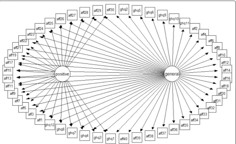
Several approaches have been suggested to model vari-ance specific to methods factors [24, 25]. To accommo-date the possible influences of such item wording effects when seeking the relevant estimates for the main con-struct of general psychological distress (GPD) we elected to apply a so-called M-1 model [25]. This model as-sumes the existence of a general factor as well as M-1 method latent variables where M stands for specific (nuisance) factors explaining the common variance of items sharing the same wording. In the framework of our study, the M-1 model translates into the general fac-tor accounting for shared variance (here GPD) across all 52 items in our item bank and one specific factor ac-counting for positively worded items from both mea-sures1. Figure 1 provides a graphical representation of the M-1 model.
To demonstrate the relevance of a bifactor approach for our data, we compare its fit to data with a unidimensional solution, i.e. a solution where all items load on a general factor and no specific factors are included. For evaluation of model fit, traditional fit indices were used, including Satorra-Bentler scaled chi-square [28], comparative fit index (CFI) [29], Tucker-Lewis fit index (TLI) [30] and root mean square error of approximation (RMSEA) [31]. Cor-rectedχ2difference test was used for the comparison [32]. All models were estimated with MPlus [33] using mean and variance adjusted Weighted Least Squares (WLSMV) estimation. Therefore the resulting model can be referred as the normal ogive Graded Response Model (GRM) [34, 35].
CAT simulation
αim¼ ffiffiffiffiffiffiffiffiffiffiffiffiffiffiffiffiffiffi1:7λim 1−
XM
m¼1 λ2
im
s andtik ¼ ffiffiffiffiffiffiffiffiffiffiffiffiffiffiffiffiffiffi1:7τik
1−
XM
m¼1 λ2
im
s ,
whereλimis factor loading of the item on factorm,τik are the corresponding item thresholds and the scaling constant 1.7 converts estimates from the normal ogive metric of the factor model into logistic IRT metric needed for the CAT application.
To evaluate the performance of the proposed item bank we set up a Monte Carlo simulation. The simulation can be used to evaluate the efficacy of CAT administration and also the proximity of the latent factor values from the CAT administration (θest) to the true latent factor values (θtrue). In such a setting, a matrix of item parameter estimates from a calibration study and a vector of values ofθtrueneed to be provided. Also, the IRT model has to be specified. The process can be outlined as follows:
1. Simulate latent factor values from the desired distribution (θtrue) which serve as“true”latent distress values of the simulated respondents.
For the purposes of our simulation we first simulated 10,000 θtrue values from standard normal distribution N(0,1) which is the presumed empirical distribution of
distress in the general population. These values are there-fore used to investigate the functioning of the item bank in its epidemiological context. We also ran a second simula-tion based on 10,000θtruevalues drawn from uniform dis-tribution U(-3,3). Although such a disdis-tribution of distress is unlikely in the general population, the rationale is to elim-inate the influence of the empirical distribution of the latent factor on CAT performance.
2. Supply item parameter estimates and choose the corresponding IRT model.
In the context of our study, this step means to supply IRT parameters (discriminations and item thresholds) from item calibration and define which model was used for the calibration (normal ogive GRM in our case). To-gether with the θtrue values simulated from the previous step, this provides the information needed for a simu-lated CAT administration, because stochastic responses to the items can be generated (see step 4).
3. Set CAT administration options
criteria and other CAT specific settings. It requires careful selection of manipulated options since other-wise the number of cells in the simulation design in-creases rapidly. In our simulation, we aimed to evaluate the performance of the item bank in combination with the following:
Latent factor (θ) estimators [37]:
a. Maximum likelihood estimation (MLE) b. Bayesian modal estimation (BME) c. Expected A Priori estimation (EAP).
Item selection methods:
a. unweighted Fisher information (UW-FI) [38,39] b. pointwise Kullback-Leibler divergence (FP-KL) [40]:
For more details about implementation of these algo-rithms please see [41]
Priors for the distribution ofθin the population (only for BME and EAP):
a. (standard) normal b. uniform.
Termination criteria (whichever comes first): a) standard error of measurement thresholds: 0.25; 0.32; 0.40, 0.45, 0.50 or b) all items are administered.
This resulted in the 50 cells in the simulation design matrix. The following settings were kept constant across all cells:
Initialθstarting values: random draws from U(-1,1)
Number of items selected for starting portion of CAT: 3
Number of the most informative items from which the function randomly selects the next item of CAT: 1 (i.e. the most informative item is always selected).
Additional parameters can be added to control the frequency of item selection (indeed most informative items tend to be selected too often and the least inform-ative are selected rarely – this issue is known as item exposure). We do not control for item exposure in our study as it is not considered (yet) to be of great concern in mental health assessment applications, but the simu-lation study also allowed us to explore the relevance of this aspect for this item bank.
4. Simulate CAT administration
Within each of the cells of the simulation design, an administration of the item bank is simulated for each randomly generated θtrue value (from step 1). Based on an initial starting θ value, three items are chosen from the item bank (see step 3, initial θ starting values) and
stochastic responses are calculated for the respective
θtruevalues. Based on these responses, an initial estimate of the latent factor value is calculated (see step 3,θ esti-mators); for which a new item to present is selected from the item bank (see step 3, item selection methods). This process is repeated until a pre-set termination cri-terion is reached (see step 3, termination criteria). This process mimics standard CAT applications [11] and re-sults in estimates (θest) for each of the simulatedθtrue.
The CAT simulation analysis was performed in the R package catIrt [41]. Please consult its reference manual [41] for a full description of available simulation options. Key information was stored for each simulated CAT ad-ministration: which items were administered and their order, estimatedθestand its standard error after item
ad-ministration. Computer code is provided in an Add-itional file 1.
CAT performance was assessed by means of the num-ber of administered items, mixing of items from GHQ-12 and Affectometer-2 during CAT administration, and by the proximity ofθestfrom CAT administration to the simulated θtrue. Such proximity can be evaluated based on the root mean squared error, computed as
RMSE¼
ffiffiffiffiffiffiffiffiffiffiffiffiffiffiffiffiffiffiffiffiffiffiffiffiffiffiffiffiffiffiffiffiffi
1 n
X
θest−θtrue
ð Þ2
q
.
Thus, values can be interpreted as the standard devi-ation of the differences (on the logit scale) between the CAT estimated and the trueθs. We also present correla-tions between these two quantities. Lower values of RMSE and correlations closer to unity indicate better performance.
Results
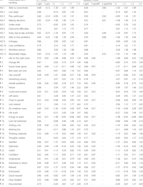
The left half of Table 1 presents factor loadings and thresholds of the M-1 model. Although χ2 indicates significant misfit (χ2= 4653, df = 1248, p< 0.001), other fit indices indicate marginal fit (CFI = 0.922; TLI = 0.917, RMSEA = 0.063). This model showed significant im-provement in model fit when compared to the unidi-mensional solution (χ2 difference = 948, df = 26, p< 0.001).
Table 1Factor loadings (λ) and thresholds (τ) of GHQ-12 and Affectometer-2 items
Item Abbreviated item wording
M-1 model Updated model
λgen λpos τ1 τ2 τ3 τ4 λgen λposAff λposGHQ τ1 τ2 τ3 τ4
GHQ 1 Able to concentrate 0.68 −0.12 −1.30 1.01 1.89 - 0.58 - 0.60 −1.30 1.01 1.89
-GHQ 2 Lost sleep 0.66 - −0.14 0.87 1.59 - 0.67 - - −0.14 0.87 1.59
-GHQ 3 Play useful part 0.60 −0.14 −0.99 1.24 1.91 - 0.50 - 0.54 −0.99 1.24 1.91
-GHQ 4 Making decisions 0.65 −0.24 −1.08 1.40 2.14 - 0.52 - 0.61 −1.08 1.40 2.14
-GHQ 5 Under strain 0.73 - −0.45 0.76 1.63 - 0.74 - - −0.45 0.76 1.63
-GHQ 6 Overcome difficulties 0.76 - 0.01 1.15 1.75 - 0.77 - - 0.01 1.15 1.75
-GHQ 7 Enjoy day-to-day activities 0.65 −0.15 −1.24 0.97 1.75 - 0.56 - 0.49 −1.24 0.97 1.75
-GHQ 8 Able to face problems 0.64 −0.22 −1.06 1.30 2.04 - 0.50 - 0.68 −1.06 1.30 2.04
-GHQ 9 Unhappy 0.86 - 0.00 0.93 1.62 - 0.87 - - 0.00 0.93 1.62
-GHQ 10 Lose confidence 0.79 - 0.14 1.02 1.77 - 0.81 - - 0.14 1.02 1.77
-GHQ 11 Worthless person 0.86 - 0.58 1.38 1.98 - 0.88 - - 0.58 1.38 1.98
-GHQ 12 Reasonably happy 0.63 −0.14 −1.01 1.10 1.89 - 0.54 - 0.53 −1.01 1.10 1.89
-Aff 1 Life on the right track 0.70 0.43 −1.08 0.00 0.53 1.29 0.68 0.46 - −1.08 0.00 0.53 1.29
Aff 2 Change life 0.67 - −0.83 0.14 0.74 1.64 0.68 - - −0.83 0.14 0.74 1.64
Aff 3 Future looks good 0.62 0.44 −1.27 −0.11 0.48 1.32 0.60 0.47 - −1.27 −0.11 0.48 1.32
Aff 4 Best years are over 0.63 - −0.01 0.66 1.16 1.67 0.64 - - −0.01 0.66 1.16 1.67
Aff 5 Like yourself 0.48 0.49 −1.01 −0.06 0.57 1.36 0.46 0.50 - −1.01 −0.06 0.57 1.36
Aff 6 Something wrong 0.77 - 0.27 0.91 1.41 2.10 0.78 - - 0.27 0.91 1.41 2.10
Aff 7 Handle problems 0.48 0.36 −0.85 0.18 0.75 1.53 0.45 0.40 - −0.85 0.18 0.75 1.53
Aff 8 Failure 0.88 - 0.39 1.07 1.46 2.22 0.89 - - 0.39 1.07 1.46 2.22
Aff 9 Loved and trusted 0.53 0.51 −0.45 0.54 1.02 1.64 0.51 0.53 - −0.45 0.54 1.02 1.64
Aff 10 Left alone 0.61 - 0.28 0.95 1.47 2.22 0.62 - - 0.28 0.95 1.47 2.22
Aff 11 Close to people 0.52 0.54 −0.48 0.56 0.99 1.81 0.50 0.57 - −0.48 0.56 0.99 1.81
Aff 12 Lost interest 0.72 - 0.56 1.12 1.77 2.62 0.73 - - 0.56 1.12 1.77 2.62
Aff 13 Do whatever want 0.49 0.33 −1.26 −0.39 0.28 0.97 0.46 0.37 - −1.26 −0.39 0.28 0.97
Aff 14 Life stuck 0.81 - −0.27 0.56 1.04 1.67 0.82 - - −0.27 0.56 1.04 1.67
Aff 15 Energy to spare 0.42 0.21 −1.98 −0.92 −0.08 0.83 0.40 0.27 - −1.98 −0.92 −0.08 0.83
Aff 16 Can’t be bothered 0.66 - −0.68 0.46 1.08 2.14 0.67 - - −0.68 0.46 1.08 2.14
Aff 17 Smiling a lot 0.58 0.30 −1.33 0.04 0.65 1.62 0.56 0.35 - −1.33 0.04 0.65 1.62
Aff 18 Nothing fun 0.69 - −0.11 0.80 1.33 2.01 0.70 - - −0.11 0.80 1.33 2.01
Aff 19 Thinking creatively 0.53 0.48 −1.19 0.02 0.66 1.58 0.51 0.50 - −1.19 0.02 0.66 1.58
Aff 20 Thoughts useless 0.76 - −0.03 0.65 1.27 2.10 0.77 - - −0.03 0.65 1.27 2.10
Aff 21 Satisfied 0.66 0.47 −1.37 −0.02 0.60 1.63 0.64 0.50 - −1.37 −0.02 0.60 1.63
Aff 22 Optimistic 0.44 0.44 −1.44 −0.16 0.43 1.36 0.43 0.43 - −1.44 −0.16 0.43 1.36
Aff 23 Useful 0.51 0.41 −1.13 0.18 0.82 1.70 0.49 0.45 - −1.13 0.18 0.82 1.70
Aff 24 Confident 0.62 0.45 −1.17 0.05 0.71 1.59 0.61 0.47 - −1.17 0.05 0.71 1.59
Aff 25 Understood 0.41 0.41 −1.28 0.01 0.79 1.58 0.40 0.41 - −1.28 0.01 0.79 1.58
Aff 26 Interested in others 0.40 0.46 −0.77 0.40 0.92 1.74 0.37 0.50 - −0.77 0.40 0.92 1.74
Aff 27 Relaxed 0.67 0.29 −1.37 −0.10 0.56 1.48 0.66 0.31 - −1.37 −0.10 0.56 1.48
Aff 28 Enthusiastic 0.55 0.46 −1.51 −0.18 0.50 1.50 0.53 0.50 - −1.51 −0.18 0.50 1.50
Aff 29 Good natured 0.46 0.45 −0.85 0.47 1.09 2.18 0.43 0.49 - −0.85 0.47 1.09 2.18
Aff 30 Clear headed 0.53 0.48 −0.86 0.29 0.82 1.67 0.51 0.49 - −0.86 0.29 0.82 1.67
difference = 321, df = 1,p< 0.001). This model was statisti-cally better motivated given the high loadings for the posi-tively worded GHQ-12 items (on the corresponding specific factor). Finally, this model showed better fit in comparison to the unidimensional model (χ2difference = 1320, df = 27, p< 0.001). Factor loadings and thresholds are presented in the right half of Table 1.
The correlation between the two factors accounting for positively worded items was statistically significant (p= 0.003) though small (0.143) suggesting relative inde-pendence of the positive wording method factors in GHQ-12 and Affectometer-2. Item loadings for both measures on the general factor were, with the exception of Affectometer-2 item“Interested in others”(Aff 26), all larger than 0.4 which has been suggested as a reasonable cutoff value [42]. This suggests that all covariances of items in our item bank could be explained to a reason-able extent by the single latent factor hypothesized as a population continuum of “general psychological dis-tress”. This interpretation is supported by an ωH= .90,
which indicates that responses are dominated by this single general factor [18, 36, 43].
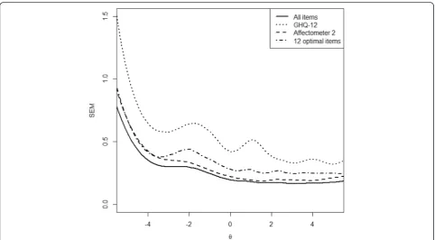
After the joint calibration on the general factor, it is possible to compare the conditional standard error of measurement (SEM) for the general factor when using either all items or specific subsets of items from the item bank. The comparison of measurement errors of individual instruments revealed that both the GHQ-12 and the Affectometer-2 were best suited to assess more distressed states: Factor estimates above the population mean (“0” in Fig. 2, i.e. more distressed individuals), were associated with a lower standard error of meas-urement and thus more precisely assessed. The differ-ence between these two item sets was mainly due to their differences in test length as well as the number of response categories (both favour the Affectometer-2). Figure 2 also shows the conditional measurement error for those 12 items from the 52-item bank that are opti-mally targeted at each distress level to explore whether the item bank improves upon the GHQ-12. In steps of
0.15 along the GPD continuum (x-axis) those 12 items with the highest information function for each specific distress level were selected and their joint information
I(θ) was converted into the conditional measurement error ( 1=pffiffiffiffiffiffiffiffiffiIð Þθ ). The resulting conditional standard error is presented as the dash-dotted line and it illus-trates the gain in measurement precision by using items from more than one instrument: in the slightly artificial case of having to choose an optimal 12 item version it is neither the widely relied-upon item set of the GHQ-12 that is chosen, nor is it only Affectometer-2 items with more response categories. Instead, this scenario already illustrates that different items can be of differ-ent value for specific assessmdiffer-ent purposes and levels of distress. In the following simulation study we assessed this question more generally as well as methodological questions comparing different selection and estimation algorithms for adaptive situations.
The solid line in Fig. 2 shows measurement error along distress levels of the combined instruments. It can also be viewed as a justification for our most stringent termination criteria with respect to SEM in our simula-tion (see Methods secsimula-tion): SEM values below 0.25 can-not be achieved with this item bank and therefore it makes little sense to include them in the simulation.
Transformation of factor analytic estimates into relevant IRT parameters
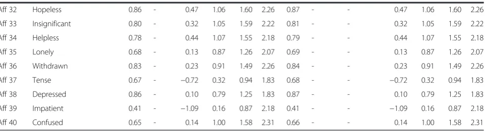
For the final model considered in our item bank, negative items load on the general factor (distress) only but positive items load on both the general as well as one of the method factor (posGHQ and posAff respectively). There-fore, the number of dimensions for negative items isM= 1 but for positive itemsM= 2. As noted previously, to elim-inate the influence of item wording, we considered and converted IRT estimates only for the general factor in this model (CAT algorithms for item banks where specific fac-tors are deemed to add further substantive information appear elsewhere [44]). Converted IRT estimates of the items included in our bank are presented in Table 2. Table 1Factor loadings (λ) and thresholds (τ) of GHQ-12 and Affectometer-2 items(Continued)
Aff 32 Hopeless 0.86 - 0.47 1.06 1.60 2.26 0.87 - - 0.47 1.06 1.60 2.26
Aff 33 Insignificant 0.80 - 0.32 1.05 1.59 2.22 0.81 - - 0.32 1.05 1.59 2.22
Aff 34 Helpless 0.78 - 0.44 1.07 1.55 2.18 0.79 - - 0.44 1.07 1.55 2.18
Aff 35 Lonely 0.68 - 0.13 0.87 1.26 2.07 0.69 - - 0.13 0.87 1.26 2.07
Aff 36 Withdrawn 0.83 - 0.23 0.91 1.49 2.26 0.84 - - 0.23 0.91 1.49 2.26
Aff 37 Tense 0.67 - −0.72 0.32 0.94 1.83 0.68 - - −0.72 0.32 0.94 1.83
Aff 38 Depressed 0.86 - 0.10 0.79 1.25 1.83 0.87 - - 0.10 0.79 1.25 1.83
Aff 39 Impatient 0.41 - −1.09 0.16 0.87 2.18 0.41 - - −1.09 0.16 0.87 2.18
CAT simulation
We used IRT parameters from Table 2 and a vector of 10,000 values ofθtruesampled from the standard normal and uniform distributions as an input for our simulation. We then manipulated (1) θ estimator, (2) item selection method, (3) termination criteria and (4) prior informa-tion on distress distribuinforma-tion in the populainforma-tion (for BME and EAP estimators).
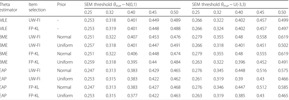
To evaluate the efficacy of CAT administration we present the number of administered items needed to reach >the desired termination criteria in Table 3. The results indicate that, to reach a high measurement precision [45, 46] of the score (i.e. standard error of measurement (SEM) = 0.25), 23–30 items on average need to be admin-istered regardless ofθestimator, item selection method, or
θtrue distribution. Not surprisingly, the number of items needed decreases dramatically as the desired SEM cutoff increases (and thus measurement precision decreases). For example, when the desired SEM cutoff is 0.32, CAT administration requires on average 10–15 items; and only 4–7 items are required for a SEM cutoff of 0.45. It is not surprising that maximum likelihood-based and Bayesianθ estimators with non-informative (uniform) priors are simi-larly effective since they are formally equivalent. However, the normal prior helps to further decrease the number of administered items, even for uniformly distributed θtrue values. Information-based and Kullback-Leibler item se-lection algorithms are similarly effective.
Table 4 shows the mixing of items from both GHQ-12 and Affectometer-2 when jointly used for CAT adminis-tration. Such mixing is relatively stable across all scenar-ios for high measurement precisions. The variability across scenarios increases with decreasing demands for measurement precision. Note, that the percentage of GHQ-12 items within the item bank was 23.1 %. We emphasize that neither item exposure control nor con-tent balancing was used in our simulations.
Values of RMSE between final θ estimates from CAT administration (θest) and their corresponding values of
θtrueare provided in Table 5.
Results show that the square root of mean square deviations between the true and estimated θ values lies between 0.247 and 0.619 logit (i.e. between 0.15 and 0.36 standard deviation).
Another traditional approach for evaluating the proximity of the estimated and true θs is the correlation coefficient. Figure 3 therefore provides scatterplots ofθtrueon the x-axis and the final estimatesθestfrom the CAT administration on the y-axis (for the UW-FI method of item selection).
The red line represents perfect correlation between
θtrue and θest, the blue one shows the fitted regression line. Figure 3 also shows no systematic bias of CAT esti-mated θs for all SEM cutoffs (dots are distributed sym-metrically along the red line). As expected, correlation is lower as the measurement precision decreases, though it is still around 0.9 even for a SEM cutoff of 0.50.
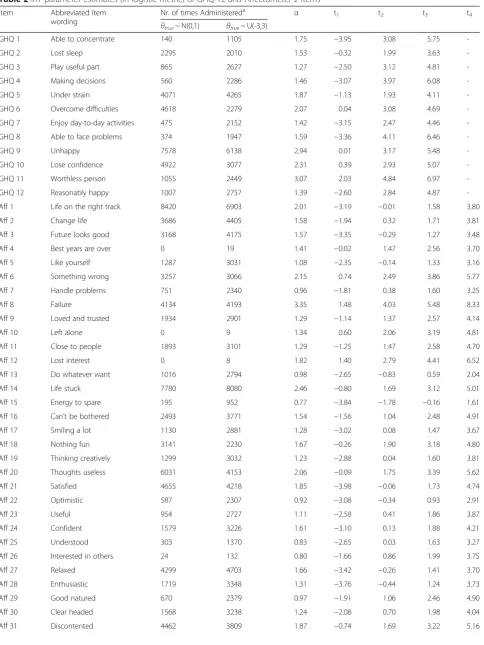
Table 2IRT parameter estimates (in logistic metric) of GHQ-12 and Affectometer-2 items
Item Abbreviated item
wording
Nr. of times Administereda α t1 t2 t3 t4
θtrue~ N(0,1) θtrue~ U(-3,3)
GHQ 1 Able to concentrate 140 1105 1.75 −3.95 3.08 5.75
-GHQ 2 Lost sleep 2295 2010 1.53 −0.32 1.99 3.63
-GHQ 3 Play useful part 865 2627 1.27 −2.50 3.12 4.81
-GHQ 4 Making decisions 560 2286 1.46 −3.07 3.97 6.08
-GHQ 5 Under strain 4071 4265 1.87 −1.13 1.93 4.11
-GHQ 6 Overcome difficulties 4618 2279 2.07 0.04 3.08 4.69
-GHQ 7 Enjoy day-to-day activities 475 2152 1.42 −3.15 2.47 4.46
-GHQ 8 Able to face problems 374 1947 1.59 −3.36 4.11 6.46
-GHQ 9 Unhappy 7578 6138 2.94 0.01 3.17 5.48
-GHQ 10 Lose confidence 4922 3077 2.31 0.39 2.93 5.07
-GHQ 11 Worthless person 1055 2449 3.07 2.03 4.84 6.97
-GHQ 12 Reasonably happy 1007 2757 1.39 −2.60 2.84 4.87
-Aff 1 Life on the right track 8420 6903 2.01 −3.19 −0.01 1.58 3.80
Aff 2 Change life 3686 4405 1.58 −1.94 0.32 1.71 3.81
Aff 3 Future looks good 3168 4175 1.57 −3.35 −0.29 1.27 3.48
Aff 4 Best years are over 0 19 1.41 −0.02 1.47 2.56 3.70
Aff 5 Like yourself 1287 3031 1.08 −2.35 −0.14 1.33 3.16
Aff 6 Something wrong 3257 3066 2.15 0.74 2.49 3.86 5.77
Aff 7 Handle problems 751 2340 0.96 −1.81 0.38 1.60 3.25
Aff 8 Failure 4134 4193 3.35 1.48 4.03 5.48 8.33
Aff 9 Loved and trusted 1934 2901 1.29 −1.14 1.37 2.57 4.14
Aff 10 Left alone 0 9 1.34 0.60 2.06 3.19 4.81
Aff 11 Close to people 1893 3101 1.29 −1.25 1.47 2.58 4.70
Aff 12 Lost interest 0 8 1.82 1.40 2.79 4.41 6.52
Aff 13 Do whatever want 1016 2794 0.98 −2.65 −0.83 0.59 2.04
Aff 14 Life stuck 7780 8080 2.46 −0.80 1.69 3.12 5.01
Aff 15 Energy to spare 195 952 0.77 −3.84 −1.78 −0.16 1.61
Aff 16 Can’t be bothered 2493 3771 1.54 −1.56 1.04 2.48 4.91
Aff 17 Smiling a lot 1130 2881 1.28 −3.02 0.08 1.47 3.67
Aff 18 Nothing fun 3141 2230 1.67 −0.26 1.90 3.18 4.80
Aff 19 Thinking creatively 1299 3032 1.23 −2.88 0.04 1.60 3.81
Aff 20 Thoughts useless 6031 4153 2.06 −0.09 1.75 3.39 5.62
Aff 21 Satisfied 4655 4218 1.85 −3.98 −0.06 1.73 4.74
Aff 22 Optimistic 587 2307 0.92 −3.08 −0.34 0.93 2.91
Aff 23 Useful 954 2727 1.11 −2.58 0.41 1.86 3.87
Aff 24 Confident 1579 3226 1.61 −3.10 0.13 1.88 4.21
Aff 25 Understood 303 1370 0.83 −2.65 0.03 1.63 3.27
Aff 26 Interested in others 24 132 0.80 −1.66 0.86 1.99 3.75
Aff 27 Relaxed 4299 4703 1.66 −3.42 −0.26 1.41 3.70
Aff 28 Enthusiastic 1719 3348 1.31 −3.76 −0.44 1.24 3.73
Aff 29 Good natured 670 2379 0.97 −1.91 1.06 2.46 4.90
Aff 30 Clear headed 1568 3238 1.24 −2.08 0.70 1.98 4.04
Discussion
The development of an item bank for measurement of psy-chological distress is a timely challenge amid public mental health debates over measuring happiness /well-being or de-pression [47–51]. In this paper we have presented, to our knowledge, the first calibration of items to measure GPD
“adaptively” focusing on practical issues in the transition from multi-instrument paper and pencil assessments to modern adaptive ones based on item banks created from
existing validated items. We chose the GHQ-12 and the Affectometer-2 because they are close in terms of content, and target population [16] but were derived differently. We have demonstrated that their items measure a common di-mension, which is in keeping with others’prior notions of general psychological distress. Potentially more instru-ments targeting the same or similar constructs can be combined to develop large item banks desirable for adap-tive testing. Thus, we do not necessarily need to invent new instruments or items - we can instead combine exist-ing and validated ones2.
Importantly, the combination of both instruments leads to an item bank which is more efficient than using
either instrument on its own. Compared to the GHQ-12, using the same number of items results in a higher measurement precision (dash-dotted line in Fig. 2) and compared to the Affectometer-2 a smaller number of items will result in sufficient measurement precision for a broad range of distress levels and assessment applica-tions. In addition, although the Affectometer-2 already consists of 40 items, the simulation study (Table 4) shows that the GHQ-12 complements its coverage of the latent construct. These can be seen as considerable advantages over the traditional use of single instruments. Pooling and calibration of this relatively small set of items required subtle analytic considerations regarding positive wording of items present in both GHQ-12 and Affectometer-2. To eliminate the influence of wording effects on our general factor we used the M-1 modelling approach [25]. A model with a single method factor accounting for the positive wording used by items in both measures was compared to an alternative model with separate method factors for positively worded items in the GHQ-12 and Affectometer-2. Low method factor loadings of GHQ-12 items and only marginal fit of the Table 2IRT parameter estimates (in logistic metric) of GHQ-12 and Affectometer-2 items(Continued)
Aff 32 Hopeless 2079 3000 3.02 1.63 3.67 5.55 7.84
Aff 33 Insignificant 2923 2417 2.32 0.93 3.02 4.58 6.39
Aff 34 Helpless 2409 2541 2.22 1.23 2.98 4.33 6.08
Aff 35 Lonely 0 9 1.64 0.31 2.04 2.98 4.89
Aff 36 Withdrawn 5565 5027 2.59 0.71 2.82 4.62 7.02
Aff 37 Tense 2763 3937 1.58 −1.67 0.75 2.19 4.24
Aff 38 Depressed 7865 6862 3.00 0.36 2.72 4.30 6.30
Aff 39 Impatient 40 231 0.77 −2.03 0.29 1.62 4.07
Aff 40 Confused 0 10 1.49 0.32 2.27 3.56 5.23
a
Number of times the items was administered out of 10,000 simulated CAT administration for SEM = 0.32, MLE and UW-FI item selection algorithm
Table 3Mean (standard deviation) number of administered items
Theta estimator
Item selection
Prior SEM thresholdθtrue~ N(0,1) SEM thresholdθtrue~ U(-3,3)
0.25 0.32 0.40 0.45 0.50 0.25 0.32 0.40 0.45 0.50
MLE UW-FI - 25 (13) 12 (6) 7 (3) 6 (2) 5 (2) 29 (17) 15 (9) 9 (5) 7 (3) 5 (3)
MLE FP-KL - 25 (13) 12 (6) 7 (3) 6 (2) 5 (2) 29 (17) 15 (9) 9 (5) 7 (3) 6 (3)
BME UW-FI Normal 23 (12) 10 (5) 5 (2) 4 (2) 3 (1) 28 (17) 13 (7) 7 (4) 5 (3) 4 (2)
BME UW-FI Uniform 25 (13) 12 (6) 7 (3) 6 (3) 5 (2) 29 (17) 15 (9) 9 (5) 7 (4) 6 (3)
BME FP-KL Normal 23 (12) 10 (5) 5 (2) 4 (2) 3 (1) 28 (17) 13 (7) 7 (4) 5 (3) 4 (2)
BME FP-KL Uniform 25 (13) 12 (6) 7 (3) 6 (3) 5 (2) 29 (17) 15 (9) 9 (5) 7 (4) 6 (3)
EAP UW-FI Normal 23 (12) 11 (5) 6 (2) 5 (2) 4 (1) 28 (17) 13 (7) 7 (4) 5 (3) 4 (2)
EAP UW-FI Uniform 26 (13) 13 (6) 8 (3) 6 (2) 5 (2) 30 (17) 15 (9) 9 (4) 7 (3) 6 (2)
EAP FP-KL Normal 23 (12) 11 (5) 6 (2) 5 (2) 4 (1) 28 (17) 13 (7) 7 (4) 5 (3) 4 (2)
former model suggest the superiority of the latter model. Interestingly, results show the positive factors from each measure to be relatively independent.
A large literature has considered the potential multidi-mensionality of the GHQ-12 [52–54]. Usually two corre-lated factors, one for positive and one for negative items, have been reported. Some authors have interpreted this finding as evidence for the GHQ-12 measuring positive and negative mental health. Others have voiced the con-cern that the second factor is mostly a methods artifact [55] due to item wording. Our item response theory based factor analysis suggests that it probably is not the former, because if the items of the GHQ-12 and the Affectometer-2 were designed to assess positive mental health with the positively phrased items and mental distress with the negatively phrased ones, then this should be mirrored by a two-factor solution across both instruments. Instead, in our models, GHQ-12 and Affectometer-2 need separate method factors to explain left-over variance in the posi-tively phrased items. This suggests that there is little sup-port for either the same response tendency or the same
latent construct underlying the positively worded items across both instruments. This is an important finding, since it indicates first that both instruments, across all their items, assess a single dimension and secondly, that the additional variance in the positively phrased items needs at least two relatively uncorrelated variables as an adequate explanatory model. There is of course interest in exactly what these factors capture, but this is difficult to say without external validation data [8]. It could be, for ex-ample, that one of them actually is a pure methods factor, while the other captures a component of positive affect [56, 57]. How relevant this latter question is, remains to be seen, since our results improve further on the current state of this debate: A reliability estimate of ωH= .90 for
the general psychological distress factor highlights that the systematic variance connected with the positively phrased items of both instruments comprises only a marginal pro-portion of the total variance in responses.
Most importantly for our purposes here, it is the factor loadings on the general factor from a model with separ-ate method factors for positively worded items that were
Table 4Mean % of GHQ-12 items in the CAT administered items
Theta estimator
Item selection
Prior SEM thresholdθtrue~ N(0,1) SEM thresholdθtrue~ U(-3,3)
0.25 0.32 0.40 0.45 0.50 0.25 0.32 0.40 0.45 0.50
MLE UW-FI - 19.7 23.1 24.2 24.6 23.9 20.7 21.5 25.0 25.8 24.9
MLE FP-KL - 19.5 22.9 24.0 24.1 23.8 20.6 21.2 24.4 24.9 24.4
BME UW-FI Normal 20.4 24.8 28.1 28.1 32.7 20.7 22.0 24.5 24.9 29.0
BME UW-FI Uniform 19.5 22.3 23.0 22.1 20.8 20.6 20.6 23.5 24.1 22.9
BME FP-KL Normal 20.2 25.0 28.3 28.6 32.8 20.7 22.0 24.8 25.9 30.3
BME FP-KL Uniform 19.3 22.3 22.8 21.8 20.9 20.3 20.9 23.5 23.3 22.3
EAP UW-FI Normal 20.1 23.9 26.6 27.8 28.3 20.5 21.4 23.7 24.3 26.4
EAP UW-FI Uniform 19.5 22.5 25.0 24.9 26.0 20.7 21.2 25.4 26.8 25.1
EAP FP-KL Normal 19.9 24.0 27.1 28.0 29.4 20.5 21.6 24.2 24.6 27.4
EAP FP-KL Uniform 19.7 22.1 25.2 23.3 25.8 20.2 21.3 24.8 25.4 25.3
% of GHQ-12 items in the item bank: (12/52)*100 = 23.1 %
Table 5Root mean square errors (RMSE) between CAT estimatedθs and trueθs
Theta estimator
Item selection
Prior SEM thresholdθtrue~ N(0,1) SEM thresholdθtrue~ U(-3,3)
0.25 0.32 0.40 0.45 0.50 0.25 0.32 0.40 0.45 0.50
MLE UW-FI - 0.253 0.318 0.401 0.449 0.489 0.266 0.322 0.402 0.457 0.499
MLE FP-KL - 0.253 0.319 0.401 0.448 0.488 0.266 0.324 0.402 0.457 0.497
BME UW-FI Normal 0.251 0.322 0.407 0.453 0.476 0.279 0.355 0.48 0.558 0.619
BME UW-FI Uniform 0.257 0.318 0.401 0.447 0.491 0.266 0.318 0.401 0.451 0.502
BME FP-KL Normal 0.251 0.322 0.406 0.448 0.474 0.279 0.355 0.48 0.555 0.619
BME FP-KL Uniform 0.259 0.318 0.395 0.44 0.484 0.263 0.322 0.396 0.452 0.491
EAP UW-FI Normal 0.247 0.313 0.383 0.429 0.465 0.276 0.345 0.448 0.516 0.575
EAP UW-FI Uniform 0.253 0.315 0.383 0.422 0.462 0.261 0.319 0.39 0.43 0.466
EAP FP-KL Normal 0.247 0.313 0.383 0.427 0.468 0.276 0.346 0.447 0.512 0.585
transformed into IRT parameters to calibrate our general psychological distress (GPD) continuum. These were then used as input for our simulation of the efficacy of CAT ad-ministration of this candidate item bank. Depending on the combination ofθestimator and item selection method, the average number of items required for CAT administra-tion to reach a SEM cutoff of 0.32 typically required for studies using individual level assessment ranged from 10 to 15. The number of administered items can be further re-duced if lower precision is acceptable (see Table 3). These figures show evidence of high efficiency and therefore the usefulness of CAT administration to reduce burden on respondents. However, these results have to be judged within the CAT context and they do not provide informa-tion on the number of items needed for a self-report ap-proach to distress assessment with traditional fixed-length questionnaires. The CAT application uses a set of different questions for each respondent optimized for their respect-ive distress levels. Fixed-format questionnaires do not have this flexibility and unless they are targeted at a specific fac-tor level, they probably need to be (much) longer than the results of the CAT simulation indicate [12, 58].
In our simulation we selected frequently used options to show how different combinations of CAT settings may affect the number of administered items. In terms of efficacy, the results suggest rather similar perform-ance of most of them. However, an informative (stand-ard normal) prior helps to further reduce the number of items, especially for lower measurement precisions. Re-searchers should be cautious when specifying inform-ative priors though, as priors not corresponding with the population distribution may have an adverse effect on the number of administered items [59].
We believe that our argument and technical work are illustrative and compelling as a justification for future fieldwork. However, there are clearly some limitations of our study. It is important to recognize that the simula-tion may show slightly over-optimistic results in terms of CAT efficiency. This is because the idealized persons’ responses to items during our CAT simulation are based on modelled probabilities and thus follow precisely the item response model used for calibration. Thus the extent of model misfit from the empirical samples is not taken into account by this work. When items are calibrated using a very large sample of respondents, this is not a big issue, but our calibration sample was of only a moderate size and therefore our item bank may need re-calibration in larger empirical datasets. We are not aware of any exist-ing large dataset that allows this, but it could become a priority to explore such a dataset.
An aspect important for future content development is the GPD factor itself. Here, we offer this term over the ori-ginal terminology (“common mental disorder”) frequently associated with the GHQ because our item bank includes
Affectometer-2 items and therefore the measured con-struct is broader. Looking at the items that have been used in the past, approaches to measure GPD currently range from symptoms of mental disorders, a perspective which overlaps with the GHQ-12 tradition [60–62], to definitions based on the affective evaluation, closer to the underlying rationale of the Affectometer-2 [56, 57]. These, sometimes more deficit oriented perspectives can then be contrasted with similar assessments based on positive psychology or well-being theories [27, 63]. The interrelations of these frameworks are currently under-researched and more inte-grative research on these is needed [8, 64, 65]. It should be noted that while our analysis presents evidence for overlap between two of these positions, this does not cover all rele-vant frameworks, nor do we present evidence for predictive or differential validity of the item sets, which would have been beyond the scope of this work.
Conclusions
The CAT administration of the proposed item bank con-sisting of GHQ-12 and Affectometer-2 items is more effi-cient than the use of either measure alone and its use shows a reasonable mixing of items from each of the two measures. The approach outlined in this manuscript com-bines previous work on data integration and multidimen-sional IRT, and together with other important and similarly minded developments in the field [66–68] illustrates a pos-sible future of quick and broad assessments in epidemi-ology and public mental health.
Ethics approval and consent to participate
Not applicable.
Consent for publication
Not applicable.
Availability of data and materials
Data from these secondary data analyses of the SHEPS sample were supplied by the UK Data Archive (study number SN5713) and can be accessed at https://disco-ver.ukdataservice.ac.uk.
Endnotes 1
The selection of modelling a specific factor for nega-tively or posinega-tively worded items is arbitrary and de-pends on the selection of “reference wording”. We selected the negative wording as our reference type of wording.
2
Additional file
Additional file 1:R code for CAT simulation (DOCX 23.7 kb)
Abbreviations
BME:bayesian modal estimation; CAPI: computer assisted personal interviewing; CAT: computerized adaptive testing; CFI: comparative fit index; CMD: common mental disorder; EAP: Expected A Priori; FP-KL: pointwise Kullback-Leibler divergence; GHQ: General Health Questionnaire;
GPD: general psychological distress; GRM: graded response model; IRT: item response theory; MLE: maximum likelihood estimation; RMSE: root mean squared error; RMSEA: root mean square error of approximation; SEM: standard error of measurement; SHEPS: Scottish Health Education Population Survey; TLI: Tucker-Lewis index; UW-FI: unweighted Fisher information; WLSMV: mean and variance adjusted Weighted Least Squares.
Competing interest
TJC reports grants from GL Assessment (2008-2011) held whilst at the University of Cambridge (with Prof J Rust) for an ability test standardization project. TJC and JS report a personal fee from GL Assessment for psychometric calibration of the BAS3 (ability tests) outside the submitted work. GL Assessment sell the General Health Questionnaire.
JB and KP declare that they have no competing interests.
Authors’contributions
Analysis and interpretation of data, drafting and revision of the article–JS; drafting and revision of the article - JRB; revision of the article - KP; drafting and revision of the article, suggestion to jointly calibrate GHQ-12 and Affectometer-2 as an item bank–TJC; critical revision for important intellectual content–all authors. All authors read and approved the final manuscript.
Acknowledgements
Not applicable.
Funding
This work was conducted whilst JS was funded by the Medical Research Council (MRC award reference MR/K006665/1), partly also by Charles University PRVOUK programme nr. P38. JS was supported by NIHR CLAHRC East of England.
Author details
1Department of Health Sciences, University of York, York, UK.2Department of
Psychiatry, University of Cambridge, Cambridge Biomedical Campus, Box 189, Cambridge CB2 0QQ, UK.3Department of Kinanthropology, Charles
University, Prague, Czech Republic.4Hull York Medical School (HYMS),
University of York, York, UK.5Dundee Centre for Health And Related
Research, School of Nursing & Health Sciences, University of Dundee and Academic Health Science Partnership Tayside, Dundee, UK.
Received: 15 January 2016 Accepted: 10 May 2016
References
1. Goldberg DP, Williams P. A user's guide to the General Health Questionnaire. Windsor UK: NFER-Nelson; 1988.
2. McDowell I. Measuring health: A guide to rating scales and questionnaires. New York: Oxford University Press; 2006.
3. Stewart-Brown S. Defining and measuring mental health and wellbeing. In: Knifton L, Quinn N, editors. Public mental health: global perspectives. edn. New York: McGraw Hill Open University Press; 2013. p. 33–42.
4. Lindert J, Bain PA, Kubzansky LD, Stein C. Well-being measurement and the WHO health policy Health 2010: systematic review of measurement scales. Eur J Public Health. 2015;25(4):731–40.
5. Wahl I, Löwe B, Bjorner JB, Fischer F, Langs G, Voderholzer U, Aita SA, Bergemann N, Brähler E, Rose M. Standardization of depression measurement: a common metric was developed for 11 self-report depression measures. J Clin Epidemiol. 2014;67(1):73–86
6. Weich S, Brugha T, King M, McManus S, Bebbington P, Jenkins R, Cooper C, McBride O, Stewart-Brown S. Mental well-being and mental illness: findings
from the Adult Psychiatric Morbidity Survey for England 2007. Br J Psychiatry. 2011;199(1):23–8.
7. Gibbons RD, Perraillon MC, Kim JB. Item response theory approaches to harmonization and research synthesis. Health Serv Outcomes Res Methodol. 2014;14(4):213–31.
8. Böhnke JR, Croudace TJ. Calibrating well-being, quality of life and common mental disorder items: psychometric epidemiology in public mental health research. Br J Psychiatry. 2015. doi:10.1192/bjp.bp.115. 165530.
9. Hussong AM, Curran PJ, Bauer DJ. Integrative data analysis in clinical psychology research. Annu Rev Clin Psychol. 2013;9:61–89. 10. Bauer DJ, Hussong AM. Psychometric approaches for developing
commensurate measures across independent studies: traditional and new models. Psychol Methods. 2009;14(2):101–25.
11. Wainer H, Dorans NJ, Flaugher R, Green BF, Mislevy RJ. Computerized adaptive testing: A primer. Hillsdale, NJ: Lawrence Erlbaum; 2000. 12. Böhnke JR, Lutz W. Using item and test information to optimize targeted
assessments of psychological distress. Assessment. 2014;21(6):679–93. 13. Hankins M. The factor structure of the twelve item General Health
Questionnaire (GHQ-12): The result of negative phrasing? Clin Pract Epidemiol Ment Health. 2008;4(1):10.
14. Egberink IJL, Meijer RR. An item response theory analysis of Harter’s Self-Perception Profile for children or why strong clinical scales should be distrusted. Assessment. 2011;18(2):201–12.
15. Goldberg DP. The detection of psychiatric illness by questionnaire. London: Oxford University Press; 1972.
16. Kammann R, Flett R. Affectometer 2: A scale to measure current level of general happiness. Aust J Psychol. 1983;35(2):259–65.
17. Tennant R, Joseph S, Stewart-Brown S. The Affectometer 2: a measure of positive mental health in UK populations. Qual Life Res. 2007;16(4):687–95. 18. Reise SP. The rediscovery of bifactor measurement models. Multivar Behav
Res. 2012;47(5):667–96.
19. Gibbons RD, Bock RD, Hedeker D, Weiss DJ, Segawa E, Bhaumik DK, Kupfer DJ, Frank E, Grochocinski VJ, Stover A. Full-Information item bifactor analysis of graded response data. Appl Psych Meas. 2007;31(1):4–19.
20. Gibbons R, Hedeker D. Full-information item bi-factor analysis. Psychometrika. 1992;57(3):423–36.
21. Romppel M, Braehler E, Roth M, Glaesmer H. What is the General Health Questionnaire-12 assessing?: Dimensionality and psychometric properties of the General Health Questionnaire-12 in a large scale German population sample. Compr Psychiatry. 2013;54(4):406–13.
22. Ye S. Factor structure of the General Health Questionnaire (GHQ-12): The role of wording effects. Pers Indiv Differ. 2009;46(2):197–201.
23. Wang W-C, Chen H-F, Jin K-Y. Item response theory models for wording effects in mixed-format scales. Educ Psychol Meas. 2014;75(1):157-78. 24. Pohl S, Steyer R. Modeling common traits and method effects in
multitrait-multimethod analysis. Multivar Behav Res. 2010;45(1):45–72. 25. Geiser C, Lockhart G. A comparison of four approaches to account for
method effects in latent state–trait analyses. Psychol Methods. 2012;17(2): 255–83.
26. Scotland NH. Health Education Population Survey. Colchester, Essex: UK Data Archive; 2006.
27. Tennant R, Hiller L, Fishwick R, Platt S, Joseph S, Weich S, Parkinson J, Secker J, Stewart-Brown S. The Warwick-Edinburgh Mental Well-being Scale (WEMWBS): development and UK validation. Health Qual Life Outcomes. 2007;5:63.
28. Satorra A, Bentler PM. Corrections to test statistics and standard errors in covariance structure analysis. In: von Eye A, Clogg CC, editors. Latent variables analysis: Applications for developmental research. edn. Thousand Oaks: Sage; 1994. p. 399–419.
29. Bentler PM. Comparative fit indexes in structural models. Psychol Bull. 1990; 107:238–46.
30. Tucker LR, Lewis C. A reliability coeffficient for maximum likelihood factor analysis. Psychometrika. 1973;38:1–10.
31. Steiger JH, Lind J. Statistically-based tests for the number of common factors. Paper presented at the annual Spring Meeting of the Psychometric Society in Iowa City. May 30, 1980.
33. Muthén L, Muthén B. Mplus: Statistical analysis with latent variables. Version 7.3. Los Angeles, CA: Muthén & Muthén; 1998-2016.
34. Samejima F. Estimation of latent ability using a response pattern of graded scores, Psychometric Monograph no 17. 1969.
35. Takane Y, Leeuw J. On the relationships between item response theory and factor analysis of discretized variables. Psychometrika. 1987;52(3):393–408. 36. McDonald RP. Test theory: A unified treatment. Mahwah: Lawrence Erlbaum
Associates, Inc.; 1999.
37. Baker FB, Kim SH. Item response theory: Parameter estimation techniques. New York: Marcell Dekker; 2004.
38. Veerkamp WJ, Berger MP. Some new item selection criteria for adaptive testing. J Educ Behav Stat. 1997;22(2):203–26.
39. van der Linden W. Bayesian item selection criteria for adaptive testing. Psychometrika. 1998;63(2):201–16.
40. Chang H-H, Ying Z. A global information approach to computerized adaptive testing. Appl Psych Meas. 1996;20(3):213–29.
41. Nydick SW: catIrt: An R package for simulating IRT-based computerized adaptive tests. R package version 0.4-2. http://CRAN.R-project.org/package=catIrt. In.; 2014. 42. Fliege H, Becker J, Walter OB, Bjorner JB, Klapp BF, Rose M. Development
of a computer-adaptive test for depression (D-CAT). Qual Life Res. 2005; 14(10):2277–91.
43. Zinbarg R, Revelle W, Yovel I, Li W. Cronbach’sα, Revelle’sβ, and Mcdonald’s ωH: their relations with each other and two alternative conceptualizations of reliability. Psychometrika. 2005;70(1):123–33.
44. Weiss DJ, Gibbons RD. Computerized adaptive testing with the bifactor model. In: Proceedings of the 2007 GMAC Conference on Computerized Adaptive Testing: 2007. 2007.
45. Dimitrov DM. Marginal true-score measures and reliability for binary items as a function of their IRT parameters. Appl Psych Meas. 2003;27(6):440–58. 46. Green BF, Bock RD, Humphreys LG, Linn RL, Reckase MD. Technical guidelines
for assessing computerized adaptive tests. J Educ Meas. 1984;21(4):347–60. 47. Seligman ME, Steen TA, Park N, Peterson C. Positive psychology progress:
empirical validation of interventions. Am Psychol. 2005;60(5):410–21. 48. Ryff CD. Happiness is everything, or is it? Explorations on the meaning of
psychological well-being. J Pers Soc Psychol. 1989;57(6):1069.
49. Wood AM, Taylor PJ, Joseph S. Does the CES-D measure a continuum from depression to happiness? Comparing substantive and artifactual models. Psychiatry Res. 2010;177(1):120–3.
50. Joseph S, Lewis CA. The Depression–Happiness Scale: Reliability and validity of a bipolar self‐report scale. J Clin Psychol. 1998;54(4):537–44.
51. Kammann R, Farry M, Herbison P. The analysis and measurement of happiness as a sense of well-being. Soc Indic Res. 1984;15(2):91–115.
52. Shevlin M, Adamson G. Alternative factor models and factorial invariance of the GHQ-12: a large sample analysis using confirmatory factor analysis. Psychol Assess. 2005;17(2):231–6.
53. Werneke U, Goldberg DP, Yalcin I, Ustun BT. The stability of the factor structure of the General Health Questionnaire. Psychol Med. 2000;30(4):823–9. 54. Hu Y, Stewart-Brown S, Twigg L, Weich S. Can the 12-item General Health
Questionnaire be used to measure positive mental health? Psychol Med. 2007;37(7):1005–13.
55. Molina JG, Rodrigo MF, Losilla JM, Vives J. Wording effects and the factor structure of the 12-item General Health Questionnaire (GHQ-12). Psychol Assess. 2014;26(3):1031–7.
56. Crawford JR, Henry JD. The positive and negative affect schedule (PANAS): construct validity, measurement properties and normative data in a large non-clinical sample. Br J Clin Psychol. 2004;43(Pt 3):245–65.
57. Simms LJ, Gros DF, Watson D, O’Hara MW. Parsing the general and specific components of depression and anxiety with bifactor modeling. Depress Anxiety. 2008;25(7):E34–46.
58. Emons WHM, Sijtsma K, Meijer RR. On the consistency of individual classification using short scales. Psychol Methods. 2007;12(1):105–20.
59. van der Linden WJ, Glas CAW, editors. Elements of adaptive testing. New York: Springer; 2010.
60. Urban R, Kun B, Farkas J, Paksi B, Kokonyei G, Unoka Z, Felvinczi K, Olah A, Demetrovics Z. Bifactor structural model of symptom checklists: SCL-90-R and Brief Symptom Inventory (BSI) in a non-clinical community sample. Psychiatry Res. 2014;216(1):146–54.
61. Glaesmer H, Braehler E, Grande G, Hinz A, Petermann F, Romppel M. The German version of the Hopkins Symptoms Checklist-25 (HSCL-25): Factorial structure, psychometric properties, and population-based norms. Compr Psychiatry. 2014;55(2):396–403.
62. Stochl J, Khandaker GM, Lewis G, Perez J, Goodyer IM, Zammit S, Sullivan S, Croudace TJ, Jones PB. Mood, anxiety and psychotic phenomena measure a common psychopathological factor. Psychol Med. 2015;45(07):1483–93. 63. JovanovićV. Structural validity of the Mental Health Continuum-Short Form:
The bifactor model of emotional, social and psychological well-being. Pers Indiv Differ. 2015;75:154–9.
64. Camfield L, Skevington SM. On subjective well-being and quality of life. J Health Psychol. 2008;13(6):764–75.
65. Wood AM, Tarrier N. Positive Clinical Psychology: a new vision and strategy for integrated research and practice. Clin Psychol Rev. 2010;30(7):819–29. 66. Gibbons RD, Weiss DJ, Pilkonis PA, Frank E, Moore T, Kim JB, Kupfer DJ.
Development of a computerized adaptive test for depression. Arch Gen Psychiatry. 2012;69(11):1104–12.
67. Gibbons RD, Weiss DJ, Kupfer DJ, Frank E, Fagiolini A, Grochocinski VJ, Bhaumik DK, Stover A, Bock RD, Immekus JC. Using computerized adaptive testing to reduce the burden of mental health assessment. Psych Serv. 2008;59(4):361–8.
68. Gibbons RD, Weiss DJ, Pilkonis PA, Frank E, Moore T, Kim JB, Kupfer DJ. Development of the CAT-ANX: a computerized adaptive test for anxiety. Am J Psychiatry. 2014;171(2):187–94.
• We accept pre-submission inquiries
• Our selector tool helps you to find the most relevant journal
• We provide round the clock customer support
• Convenient online submission
• Thorough peer review
• Inclusion in PubMed and all major indexing services
• Maximum visibility for your research
Submit your manuscript at www.biomedcentral.com/submit