R E S E A R C H
Open Access
Approximate method for boundary value
problems of anti-periodic type for differential
equations with ‘maxima’
Snezhana Hristova
*, Angel Golev and Kremena Stefanova
*Correspondence:
[email protected] Faculty of Mathematics and Informatics, Plovdiv University, Plovdiv, 4000, Bulgaria
Abstract
An algorithm for constructing two sequences of successive approximations of a solution of the nonlinear boundary value problem for a nonlinear differential equation with ‘maxima’ is given. The case of a boundary condition of anti-periodic type is investigated. This algorithm is based on the monotone iterative technique. Two sequences of successive approximations are constructed. It is proved both sequences are monotonically convergent. Each term of the constructed sequences is a solution of an initial value problem for a linear differential equation with ‘maxima’ and it is a lower/upper solution of the given problem. A computer realization of the algorithm is suggested and it is illustrated on a particular example.
MSC: 34K10; 34K25; 34B15
Keywords: differential equations with ‘maxima’; nonlinear boundary value problem; approximate solution; computer realization
1 Introduction
Differential equations with ‘maxima’ are adequate models of real world problems, in which the present state depends significantly on its maximum value on a past time interval (see [–], monograph []).
Note that usually differential equations with ‘maxima’ are not possible to be solved in an explicit form and that requires the application of approximate methods. In the current paper, the monotone iterative technique [, ], based on the method of lower and upper solutions, is theoretically proved to a boundary value problem for a nonlinear differential equation with ‘maxima’. The case when the nonlinear boundary function is a nondecreas-ing one with respect to its second argument is studied. This type of the boundary func-tion covers the case of an anti-periodic boundary condifunc-tion. An improved algorithm of monotone-iterative techniques is suggested. The main advantage of this scheme is con-nected with the construction of the initial conditions.
2 Preliminary notes and definitions
Let <T<∞be a given fixed point andhbe a positive constant. Consider the set
P(h,T) =u: [–h,T]→R:u∈C[–h; ],R,u∈C[,T],R.
Consider the following nonlinear differential equation with ‘maxima’:
x(t) =f
t,x(t), max
s∈[t–h,t]x(s)
fort∈[,T], ()
with a boundary condition
gx(),x(T)= , ()
and an initial condition
x(t) =x() fort∈[–h, ], ()
wherex∈R,f : [,T]×R×R→R,g:R×R→R.
In this paper, we study boundary condition () in the case when the functiong(x,y) is nondecreasing with respect to its second argumenty. So, the anti-periodic boundary value problem is a partial case of boundary condition (). Note that similar problems are investi-gated for ordinary differential equations [], delay differential equations [] and impulsive differential equations [], and some approximate methods are suggested. The presence of the maximum of the unknown function requires additionally some new comparison results, existence results as well as a new algorithm for constructing successive approxi-mations to the exact unknown solution.
Letα,β∈C([–h,T],R) be such thatα(t)≤β(t) on [–h,T]. Define the following sets:
W(α,β) =α(),β() ×α(T),β(T) ,
S(α,β) =u: [–h,T]→R:α(t)≤u(t)≤β(t) fort∈[–h,T],
(α,β) =
⎧ ⎨
⎩(t,x,y)∈[,T]×R×R:
α(t)≤x≤β(t)
max
s∈[t–h,t]α(s)≤y≤s∈max[t–h,t]β(s)
⎫ ⎬ ⎭.
Definition The functiong:W(α,β)→Ris said to be from the classL(γ,α,β) if for any v∈[α(T),β(T)] and for anyu,u∈[α(),β()] such thatu≥u, the inequalityg(u,v) – g(u,v)≤γ(u–u) holds.
Definition The functiong:W(α,β)→Ris said to be quasi-nondecreasing inW(α,β) if for anyx∈[α(),β()] and for anyy,y∈[α(T),β(T)] such thaty≤y, the inequality g(x,y)≤g(x,y) holds.
In connection with the construction of successive approximations, we will introduce a couple of quasi-solutions of boundary value problem ()-().
Definition We will say that the functionsα,β∈P(h,T) form a couple of quasi-lower and quasi-upper solutions of boundary value problem ()-(), if
α(t)≤ft,α(t), max
s∈[t–h,t]α(s)
fort∈[,T],
gα(),β(T)≤, ()
α(t) =α() fort∈[–h, ],
and
β(t)≥f
t,β(t), max
s∈[t–h,t]β(s)
fort∈[,T],
gβ(),α(T)≥, ()
β(t) =β() fort∈[–h, ].
In the proof of our main results, we will use the following lemma.
Lemma (Comparison result) Let the following conditions be fulfilled:
. The functionsM,L∈C([,T],R+)satisfy the inequality max
t∈[,T]
M(t) +L(t) ≤T–. ()
. The functionu∈P(h,T)satisfies the inequalities
u(t)≤–M(t)u(t) –L(t) min
s∈[t–h,t]u(s), t∈[,T], ()
u(t) =u()≤, t∈[–h, ]. ()
Then u(t)≤for t∈[–h,T].
Proof Assume the statement of Lemma is not true. Consider the following two cases. Case : Letu() < . According to the assumption, it follows that there existsη∈(,T) such thatu(t) < fort∈[–h,η),u(η) = andu(η– ) > .
Denotemint∈[–h,η]u(t) = –λ< , whereλis a positive constant. Let the pointξ∈[,η) be such thatu(ξ) = –λ.
According to the mean value theorem, it follows that there existsζ∈(ξ,η) such that
u(η) –u(ξ) =u(ζ)(η–ξ). ()
From inequalities –λ≤mins∈[ζ–h,ζ]u(s), –λ≤u(ζ) and (), we obtain
λ=u(η) –u(ξ) =u(ζ)(η–ξ)
≤–M(ζ)u(ζ) –L(ζ) min
s∈[ζ–h,ζ]u(s)
(η–ξ)
≤M(ζ) +L(ζ) λ(η–ξ)
Inequality () contradicts ().
Case : Letu() = . Define a functionu˜∈P(h,T) by the equalityu(t) =˜ u(t) –δ, where
δ> is a small enough constant.
Therefore,u() < and˜ u(t) satisfies inequality (). From case it follows˜ u(t)˜ ≤ for t∈[–h,T]. Take a limit asδ→ and obtainu(t)≤ fort∈[–h,T].
In our further investigations, we will use the following result for differential equations with ‘maxima’ which is a partial case of Theorem .. [].
Lemma (Existence and uniqueness) Let the following conditions be fulfilled:
. The functionQ∈C([,T],R).
. The functionsM,L∈C([,T],R)and satisfy inequality().
Then the initial value problem for a linear differential equation with ‘maxima’
u(t) =Q(t) –M(t)u(t) –L(t) max
s∈[t–h,t]u(s), t∈[,T], u(t) =u(), t∈[–h, ]
has a unique solution u(t)∈P(h,T).
3 Monotone-iterative method
We will give an algorithm for obtaining an approximate solution of the boundary value problem for a nonlinear differential equation with ‘maxima’ ()-().
Theorem Let the following conditions be fulfilled:
. The functionsα,β∈P(h,T)form a couple of quasi-lower and quasi-upper solutions of()-()such thatα(t)≤β(t)fort∈[–h,T].
. The functiong∈C(W(α,β),R)is quasi-nondecreasing inW(α,β)and g∈L(γ,α,β).
. The functionf∈C((α,β),R)and for(t,x,y), (t,x,y)∈(α,β)such that x≤x,y≤ythe inequality
f(t,x,y) –f(t,x,y)≤–M(t)[x–x] –L(t)[y–y]
holds,where the functionsM,L∈C([,T],R+)satisfy inequality(). Then there exist two sequences{αn(t)}∞n=and{βn(t)}∞n=such that
(a) The functionsαn,βn∈P(h,T)(n= , , . . .)and(αn,βn)is a couple of quasi-lower and quasi-upper solutions of boundary value problem()-().
(b) The sequence{αn(t)}∞n=is nondecreasing.
(c) The sequence{βn(t)}∞n=is nonincreasing.
(d) Fort∈[–h,T]the inequalities
α(t)≤ · · · ≤αn(t)≤βn(t)≤ · · · ≤β(t), ()
V(t) = lim
n→∞αn(t), W(t) =nlim→∞βn(t)
(e) Both sequences are uniformly convergent on[–h,T],and(V,W)is a couple of quasi-solutions of boundary value problem()-()inS(α,β).
(f ) If additionally the functionf(t,x,y)is Lipschitz in(α,β),then there exists a unique solutionu(t)of boundary value problem()-()and
limn→∞αn(t) =limn→∞βn(t) =V(t) =W(t) =u(t)fort∈[–h,T].
Proof We will give an algorithm for construction of successive approximations to the un-known exact solution of nonlinear boundary value problem ()-().
Assume the functionsαj(t) andβj(t),j= , , . . . ,n, are constructed. Then consider both initial value problems for the linear differential equations with ‘maxima’
x(t) =Qn+(t) –M(t)x(t) –L(t) max
s∈[t–h,t]x(s), t∈[,T], ()
x(t) =αn() –
γg
αn(),βn(T)
, t∈[–h, ], ()
and
y(t) =Pn+(t) –M(t)y(t) –L(t) max
s∈[t–h,t]y(s), t∈[,T], ()
y(t) =βn() –
γg
βn(),αn(T)
, t∈[–h, ], ()
where
Qn+(t) =f
t,αn(t), max s∈[t–h,t]αn(s)
+M(t)αn(t) +L(t) max s∈[t–h,t]αn(s)
and
Pn+(t) =f
t,βn(t), max s∈[t–h,t]βn(s)
+M(t)βn(t) +L(t) max s∈[t–h,t]βn(s).
According to Lemma , initial value problems (), () and (), () have unique solu-tionsαn+,βn+∈P(h,T).
So, step by step we can construct two sequences of functions{αn(t)}∞n=and{βn(t)}∞n=. Now, we will prove by induction that forj= , , , . . . ,
(H) αj+(t)≥αj(t)andβj+(t)≤βj(t)fort∈[–h,T];
(H) αj+(t)≤βj+(t)fort∈[–h,T];
(H) (αj+,βj+)is a couple of quasi-lower and quasi-upper solutions of boundary value
problem ()-().
Assume the claims (H)-(H) are satisfied forj= , , . . . ,n– . We will prove (H) forj=n.
Define the functionp∈P(h,T) by the equalityp(t) =αn(t) –αn+(t).
Lett∈[–h, ]. Then according to condition of Theorem , the inductive assumption and the definition of the functionsαn(t),αn+(t), we have
p(t) =αn–() –αn()
+
γ
gαn(),βn(T)
=αn–() –αn()
+
γ
gαn(),βn(T)
–gαn–(),βn(T)
+
γ
gαn–(),βn(T)
–gαn–(),βn–(T)
≤. ()
Lett∈[,T]. From (H) forj=n– , condition of Theorem , the definition of the functionsαn(t),αn+(t) and (), we get
p(t)≤–M(t)αn(t) –αn+(t)
–L(t) max
s∈[t–h,t]αn(s) – max
s∈[t–h,t]αn+(s)
. ()
Note that for anyt∈[,T] the following inequality holds:
max
s∈[t–h,t]αn(s) –s∈max[t–h,t]αn+(s)≥s∈min[t–h,t]
αn(s) –αn+(s) . ()
From inequalities () and () it follows
p(t)≤–M(t)p(t) –L(t) min s∈[t–h,t]p(s).
According to Lemma , we getp(t)≤ fort∈[–h,T]. Thus,αn(t)≤αn+(t) fort∈ [–h,T].
Define the functionp∈P(h,T) by the equalityp(t) =βn+(t)–βn(t). Then fort∈[–h, ] we have
p(t) =βn() –βn–()
+
γ
gβn–(),αn–(T)
–gβn(),αn(T)
=βn() –βn–()
+
γ
gβn–(),αn–(T)
–gβn(),αn–(T)
+
γ
gβn(),αn–(T)
–gβn(),αn(T)
≤. ()
From equation (), the inductive assumption, the definition of the functions βn(t),
βn+(t) and condition of Theorem , it follows the validity of the inequality
p(t)≤–M(t)p(t) –L(t) min s∈[t–h,t]p(s).
According to Lemma , we getp(t)≤ fort∈[–h,T],i.e., the claim (H) is true for j=n.
Lett∈[–h, ]. From condition of Theorem , the inductive assumption and the defi-nition of the functionsαn+(t),βn+(t), we obtain
p(t) =αn() –βn() +
γ
gβn(),αn(T)
–gαn(),αn(T)
+
γ
gαn(),αn(T)
–gαn(),βn(T)
≤.
Lett∈[,T]. According to the choice of the functionsαn+(t),βn+(t), condition of Theorem and inequality maxs∈[t–h,t]αn+(s) –maxs∈[t–h,t]βn+(s)≥mins∈[t–h,t][αn+(s) –
βn+(s)], we get
p(t)≤–M(t)p(t) –L(t) min s∈[t–h,t]p(s).
According to Lemma , it followsp(t)≤ fort∈[–h,T]. Therefore, the claim (H) is satisfied forj=n.
Now, we will prove the claim (H) forj=n. Lett∈[–h, ]. Then from () we get
αn+(t) =αn() –
γg
αn(),βn(T)
=αn+(). ()
From (H) forj=n, condition of Theorem and the choice of the functionαn+(t), we obtain
gαn+(),βn+(T)
=gαn+(),βn+(T)
–gαn(),βn+(T) +g
αn(),βn+(T)
≤γαn+() –αn() +g
αn(),βn+(T)
= –gαn(),βn(T)
+gαn(),βn+(T)
≤. ()
Lett∈[,T]. From condition of Theorem , inequalities () and (H), we get
αn+(t) = –M(t)αn+(t) –αn(t)
–L(t)
max
s∈[t–h,t]αn+(s) –s∈max[t–h,t]αn(s)
+f
t,αn+(t), max s∈[t–h,t]αn+(s)
+ft,αn(t), max s∈[t–h,t]αn(s)
–f
t,αn+(t), max s∈[t–h,t]αn+(s)
≤f
t,αn+(t), max s∈[t–h,t]αn+(s)
. ()
For any fixedt∈[–h,T], the sequences{αn(t)}n∞=and{βn(t)}∞n=are nondecreasing and nonincreasing, respectively, and they are bounded byα(t) andβ(t).
Therefore, both sequences converge pointwisely and monotonically. Letlimn→∞αn(t) = V(t) andlimn→∞βn(t) =W(t) fort∈[–h,T]. According to Dini’s theorem, both sequences converge uniformly and the functionsV(t),W(t) are continuous. Additionally, the claims (H), (H) proveV,W∈S(α,β).
Now, we will prove that for anyt∈[,T] the following equality holds:
lim
n→∞
max ξ∈[t–h,t]αn(ξ)
= max ξ∈[t–h,t]
lim
n→∞αn(ξ)
. ()
For anyt∈[,T], we introduce the notationmaxξt∈[t–h,t]αn(ξt) =An(t). From condition (H) it follows that for anyξt∈[t–h,t] the inequalitiesαn–(ξt)≤αn(ξt)≤An(t) hold and thus,An–(t)≤An(t),n= , , . . . ,i.e., the sequence{An(t)}∞n=is monotone nondecreasing and bounded from above byβ(t) for anyt∈[–h,T]. Therefore, there exists the limit A(t) =limn→∞An(t).
From the monotonicity of the sequence of the quasi-lower solutionsαn(t), we get that for ξt ∈ [t –h,t] the inequality αn(ξt)≤V(ξt) holds. Let ηt ∈ [t –h,t] be such that
maxξt∈[t–h,t]V(ξt) =V(ηt).
AssumeV(ηt) <A(ηt). Then there exists a natural numberN such that the inequal-ities V(ηt) < AN(ηt)≤ A(ηt) hold. Therefore, there exists ξt ∈ [ηt –h,ηt] such that
αN(ξt) =maxξt∈[ηt–h,ηt]αN(ξt) =AN(ηt) orV(ηt) <αN(ξt)≤V(ξt). The obtained contra-diction proves the assumption is not valid.
AssumeV(ηt) >A(ηt). According to the definition of the functionV(t), it follows that for the fixed numberηt, we havelimn→∞αn(ηt) =V(ηt). Then there exists a natural number Nsuch thatA(ηt) <αN(ηt)≤V(ηt) andmaxηt∈[t–h,t]αN(ηt) =AN(ηt). Therefore,αN(ηt)≤
maxηt∈[t–h,t]αN(ηt)≤A(ηt). The obtained contradiction proves the assumption is not valid.
Therefore, the required equality () is fulfilled.
In a similar way, we can prove that for anyt∈[,T] the equality
lim
n→∞
max ξ∈[t–h,t]βn(ξ)
= max
ξ∈[t–h,t]
lim
n→∞βn(ξ)
()
holds.
Take a limit asn→ ∞in () and get
V(t) =V() –
γg
V(),W(T) fort∈[–h, ]. ()
From () fort= , we getg(V(),W(T)) = .
Taking a limit in the integral equation equivalent to (), we obtain the functionV(t) satisfies equation () fort∈[,T].
In a similar way, we can prove that W(t) satisfies equation () for t ∈ [,T] and g(W(),V(T)) = . Therefore, the couple (V,W) is a couple of quasi-solutions of ()-() inS(α,β) such thatV(t)≤W(t) fort∈[–h,T].
Let the functionf(t,x,y) be Lipschitz. Then if () has a solutionu(t), it is unique (see []). In this case,V(t)≡W(t) and fort∈[–h,T],
lim
4 Applications
We will apply the given above algorithm for approximate solving of a nonlinear boundary value problem.
Example Consider the following nonlinear boundary value problem for a nonlinear dif-ferential equation with ‘maxima’:
u=
–u(t)– s∈max[t–.,t]u(s) –
, t∈[, .], ()
u() +u()+eu(.)= ,
u(t) =u(), t∈[–., ].
()
Boundary value problem (), () is of type ()-(), whereh= .,T = .,f(t,x,y) =
–x– y–
andg(x,y) = x+x
+ey– .
Letα(t)≡– andβ(t)≡. The couple (α(t),β(t)) is a couple of quasi-lower and quasi-upper solutions of boundary value problem (), ().
Let (t,x,x), (t,y,y)∈ {(t,u,v)∈[, .]×[–, ]×[–, ]}andxi≤yi,i= , . There-fore,
f(t,x,x) –f(t,y,y) =
x–y ( –x)( –y)
– [x–y]≤–M(t)(x–y) –L(t)(x–y),
whereM(t)≡,L(t)≡ fort∈[, .]. Thus, condition of Theorem holds.
The functiong(x,y) is quasi-nondecreasing with respect toyandg∈L(γ,α,β),γ= . The above given problem has a zero solution. We will apply the procedure given in The-orem to obtain two sequences, which are monotonically convergent to .
The functionαn(t),n≥, is a solution of problem (), (), which is reduced to the following linear initial value problem:
αn(t) = –αn(t) – max
s∈[t–.,t]αn(s) –
+
–αn–(t)
+αn–(t), t∈[, .],
αn(t) = .αn–() – .
αn–()
– .eβn–(.)+ ., t∈[–., ].
()
The functionβn(t),n≥, is a solution of problem (), (), which is reduced to the following linear initial value problem:
βn(t) = –βn(t) – max
s∈[t–.,t]βn(s) –
+
–βn–(t)
+βn–(t), t∈[, .],
βn(t) = .βn–() – .
βn–()
– .eαn–(.)+ ., t∈[–., ].
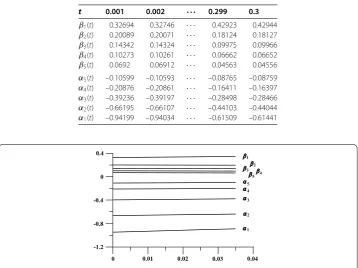
Table 1 Values of the successive approximationsαn(t) andβn(t),n= 1, 2, 3, 4, 5
t 0.001 0.002 ··· 0.299 0.3
β1(t) 0.32694 0.32746 · · · 0.42923 0.42944 β2(t) 0.20089 0.20071 · · · 0.18124 0.18127 β3(t) 0.14342 0.14324 · · · 0.09975 0.09966 β4(t) 0.10273 0.10261 · · · 0.06662 0.06652 β5(t) 0.0692 0.06912 · · · 0.04563 0.04556 α5(t) –0.10599 –0.10593 · · · –0.08765 –0.08759 α4(t) –0.20876 –0.20861 · · · –0.16411 –0.16397 α3(t) –0.39236 –0.39197 · · · –0.28498 –0.28466 α2(t) –0.66195 –0.66107 · · · –0.44103 –0.44044 α1(t) –0.94199 –0.94034 · · · –0.61509 –0.61441
Figure 1 Graphic of the successive approximationsαn(t) andβn(t),n= 1, 2, 3, 4, 5.
According to Lemma , initial value problems () and () have unique solutionsαn(t) andβn(t), respectively. Because of the presence of the maximum of the unknown func-tion over a past time interval, there is no explicit formula for the exact solufunc-tions of () and (). We use a computer program based on a modified numerical method to solve these problems (see []).
Also, by a computer realization of the scheme given in Theorem and applied to prob-lems () and (), we obtain the values in Table .
From Table and Figure , it is obvious that the sequence{αn(t)}is increasing and the sequence{βn(t)}is decreasing and both monotonically converge to the unique solution of nonlinear boundary value problem (), ().
Competing interests
The authors declare that they have no competing interests.
Authors’ contributions
Each of the authors SH, AG and KS contributed to each part of the work equally and read and proved the final version of the manuscript.
Received: 16 October 2012 Accepted: 9 January 2013 Published: 25 January 2013 References
1. Agarwal, R, Hristova, S: Strict stability in terms of two measures for impulsive differential equations with ‘supremum’. Appl. Anal.91(7), 1379-1392 (2012)
2. Bohner, M, Georgieva, A, Hristova, S: Nonlinear differential equations with ‘maxima’: parametric stability in terms of two measures. Inf. Sci. Appl. Math.7(1), 41-48 (2013)
3. Bohner, M, Hristova, S, Stefanova, K: Nonlinear integral inequalities involving maxima of the unknown scalar functions. Math. Inequal. Appl.12(4), 811-825 (2012)
5. Bainov, D, Hristova, S: Differential Equations with Maxima. Taylor & Francis/CRC, Boca Raton (2011)
6. Ladde, G, Lakshmikantham, V, Vatsala, A: Monotone Iterative Techniques for Nonlinear Differential Equations. Pitman, New York (1985)
7. Nieto, J, Yu, J, Yan, J: Monotone iterative methods for functional differential equations. Nonlinear Anal.32, 741-747 (1998)
8. Jankowski, T: Ordinary differential equations with nonlinear boundary conditions of antiperiodic type. Comput. Math. Appl.47, 1419-1428 (2004)
9. Jankowski, T: On delay differential equations with nonlinear boundary conditions. Bound. Value Probl.2005, 201-214 (2005)
10. Jankowski, T: First-order impulsive ordinary differential equations with advanced arguments. J. Math. Anal. Appl.331, 1-12 (2007)
11. Hristova, S, Stefanova, K: Linear integral inequalities involving maxima of the unknown scalar functions. Funkc. Ekvacioj53, 381-394 (2010)
12. Golev, A, Hristova, S, Rahnev, A: An algorithm for approximate solving of differential equations with ‘maxima’. Comput. Math. Appl.60, 2771-2778 (2010)
doi:10.1186/1687-2770-2013-12