http://www.sciencepublishinggroup.com/j/ijamtp doi: 10.11648/j.ijamtp.20180401.11
ISSN: 2575-5919 (Print); ISSN: 2575-5927 (Online)
An Accurate Quadrature for the Numerical Integration of
Polynomial Functions
Tahar Latrache
Department of Civil Engineering, University of Tebessa, Tebessa, Algeria
Email address:
To cite this article:
Tahar Latrache. An Accurate Quadrature for the Numerical Integration of Polynomial Functions. International Journal of Applied Mathematics and Theoretical Physics. Vol. 4, No. 1, 2018, pp. 1-7. doi: 10.11648/j.ijamtp.20180401.11
Received: December 15, 2017; Accepted: January 8, 2018; Published: January 19, 2018
Abstract:
The numerical integration of polynomial functions is one of the most interesting processes for numerical calculus and analyses, and represents thus, a compulsory step especially in finite elements analyses. Via the Gauss quadrature, the users concluded a great inconvenience that is processing at certain points which not required the based in finite element method points for deducting the form polynomials constants. In this paper, the same accuracy and efficiency as the Gauss quadrature extends for the numerical integration of the polynomial functions, but as such at the same points and nods have chosen for the determination of the form polynomials. Not just to profit from the values of the polynomials at those points and nods, but also from their first derivatives, the chosen points positions are arbitrary and the resulted deducted formulas are therefore different, as will be presented bellow and implemented.Keywords:
Integration Quadrature, Numerical Methods, Numerical Integration, Polynomial Functions, Accurate Methods1. Introduction
The Gauss quadrature represents an accurate method for the numerical integration of polynomials and by a technique of subdividing the limit integral to rectangles and in some points called Gauss points, which represent in the parametric formulation, the coordinates of the ordinates of those rectangles. The classical method represents actually an exact numerical one for the integration of polynomials and very effective for any functions. In the literature, the Gauss quadrature is known as a very precise and effective numerical integration method [1, 21], and in finite elements some elementary matrices and vectors are defined as the numerically or the theoretically of some others; in structural mechanics, the elementary stiffness matrices are deducted via the Gauss quadrature of the scalar product of the elasticity by the deformation-displacement matrices and their transpose. The deformation-displacement matrices are in general computing only once, and used to compute stiffness and strains and therefore stresses matrices and vectors, the fact which in general calls to extrapolation functions to compute those quantities at the level of nods, the main points used to express the form polynomials and thereof, the analysts needs to know the values of the
computed results at the level of.
In this new proposal, the developed method is addressed to the applied mathematics users and to the finite elements ones especially. Herein, the polynomial functions we proceed to integrate using this new approach, are defined such that their constants are related to the ordinates of these polynomials and their first derivatives at the chosen points to find the integral expression concerns and thus, the liberty to choose the number and the integral points positions is actually complete and anyway, following this method the developed formulas represent exactly the integrated polynomials with which, are related to the ordinates of these functions and their first derivatives at the points have chosen.
of the numerical parts of the formulas which called ‘weights’ and also by the ordinates or their first derivatives of multi-dimensions polynomial functions at the integral points.
Moreover, the method will be experimented by some examples and the results will be discussed.
2. Expressions of the Polynomial
Functions Constants
Suppose that is a polynomial function defined and the proceeding is to express its integral in the interval [ ]. The polynomial of the 2n-1 degree can be exactly or approximately expressed by a polynomial function of the form
⋯ ⋯ (1) And its first derivative
′ 2 ⋯ ⋯ 2 1 (2) In addition, to transform the polynomial function
defined in the interval [ ] in Cartesian coordinates to in [ 1 1], the parametric ones, it is sufficient to relate the two coordinates by the expression
(3)
Such that, (Figure 1) and the integral can be written as
(4)
Expression with which, and,
⋯ ⋯ (5) The polynomial constants can be easily deducted in
relations with , and with which , as follows Figure 1. The two points representation of in the parametric formulation.
! " # " $
2 %2& ⋯ %2& ⋯ %2&
2 2 %2& ⋯ %2&⋯ ⋯ 2 1 %2&
! #
$ ∑+, ()*+ + 0
()* ∑+, . ()*+ + 0 / 0 2 ⋯
(6)
Otherwise, in order to relate the constants with 1 and ′ 1 , it is needed to express 2 equations and integral points in the parametric formulation. For a polynomial function of the first degree, one point sufficient, and of the third degree, of two points and so on
2 1 1 1
3
1 3 1 ′1 1, 2, ⋯ , 1 0. , 1. , 1. , ⋯ (7)
Expressions, such that the fixed points in the Cartesian coordinates shall be equal, 1 ) 1 1
And,
6 1 (
)
1 1 * 1 1
3
,7 1 3() 1 1 * ) 3 1 ) ′1
(8)
1. Polynomial functions of the first degree
Suppose that the polynomial is formed by a polynomial function , such that
8 % 2 & + 2 = +
3,7
= 2 =
Thus, just only one integral point at the middle of the interval [−1 + 1] is necessary and sufficient to integrate exactly or approximately the function , such that = 0 and
2 + 0 == ′
Or,
2 = = ′ (9)
Expressions, such that ′ is the derivative of with respect to , we can therefore rewrite
= + ′ (10) 2. Polynomial functions of the third degree
The third degree polynomial functions can be given by the expression
= + + + 9 9 (11)
In Cartesian coordinates, and in parametric ones, by
= + + + 9 9 (12) Such that,
! "" # ""
$ = +) + ()* + ()*9 9 =) + 2 ()* + 3 ()*9 9
= ()* + 3 ()*9 9
9= ()* 9
9
(13)
Moreover, in order to deduct the expressions relating between , 1 and ′1, it shall resolve the linear equations system
8
+ + + 9= − + − 9=
+ 2 + 3 9= 3 − 2 + 3 9= ′
(14)
Such that and ′ are evaluated at = +1. and
= −1. respectively (the two limits of the interval), the results can be given thus by
! "" # ""
$ = ; ′ ′; < =9 ; ′ ′;
< = ′ ′;
<
9= ; < ′ ′;
(15)
Therefore, the polynomial functions (12) in relation with the expressions of (15), can be rewritten
= = =; =3 =3;
< +
9 = =; =3 =3;
< +
=3 =3; < +
= =; =3 =3;
< 9 (16)
Following the same way, via the resolution of the equations system (7), the constants of the polynomial function (5) can be then deducted and related to 1 and ′1 for superior degrees
3. The Integral Expressions of the Polynomial Functions
1. The first degree polynomials (one integral point)
For the first degree polynomial functions (10), their integral expression is the result of
> = ? = @ + 2′ A
Or
> = 2 × (17) And in Cartesian coordinates, as such
)× 2 × = × = − × ( = *
(18)
Such that is the value of at = (i.e. at = + , and = 0). 2. The third degree polynomials (two integral points)
> ? 2 +23 = 22 + − ′ − ′4 +23 ′ − ′4
Thus,
> = 1.× + −9× ′ − ′ (19)
And in the Cartesian coordinates,
> = = × DE + F −9× × E 3 − ′ FG (20)
Such that ′ is the first derivative of the function with respect to and,
H= H7 =
H H7
H=
H =
) H=
H (21)
And the multiplication factor − ⁄2 appears before, represents the Jacobean of the transformation, and appears also before the derivatives with respect to according to (21).
3. The fifth degree polynomial functions (three integral points)
In this proposed approach, the liberty is considered complete for choosing the integral points positions, and with the Gaussian fixed points positions, the derivatives parts disappeared. Also, if equal distances between points is chosen, for instance the two interval limits and its middle, the constants , and < are thus given by
=
=4 + − 8 − ′ − ′4
<=−2 + + 4 + ′ − ′4
Thus, the integral of the fifth degree polynomials, and which related to , and < by,
> = ? = 2 +23 +25 <
Can be easily simplified by the expression,
> = LM× + + NM× − M× ′ − ′ (22)
In parametric coordinates, and in the Cartesian ones by,
> = = × DLM× E + F + NM× − M× × E 3 − ′ FG (23)
4. The seventh degree polynomial functions (four integral points)
Suppose that is a seventh degree polynomial function, its exact integral in the parametric coordinates is related to , , < and N by,
> = = 2 +9 +M <+L N (24)
Otherwise, easily could be expressed as such,
> = O × + + O × E /N+ /NF + OQQQQ × ′ − ′ + OQQQQ × E ′ /N− ′ /NF (25)
Replacing and ′ by their expressions
> = O 2 + 2 + 2 <+ 2 N + O (2 +N +NR <+NS N*+OQQQQ 4 + 28 + 16 N + OQQQQ (N< +NU <+NV N*
The two expressions (25) and (24) shall be equal, and such that the following equations system is resulted
! " # "
$ O + O = 1 O +N O + 2OQQQQ +NOQQQQ =9 O +NRO + 4OQQQQ +N<UOQQQQ =M O +NSO + 6OQQQQ +NNVOQQQQ =L
(26)
! "" # ""
$ O 2O + 2O9= 2
O +<O9+ 2OQQQQ + OQQQQ =9 O +< O9+ 4OQQQQ + OQQQQ =M O +<UO9+ 6OQQQQ + 9NOQQQQ =L O +<RO9+ 8OQQQQ + 9NOQQQQ =W
(27)
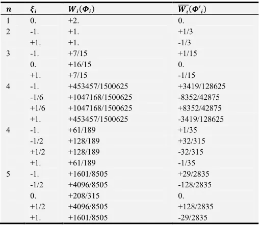
From one to five integral points, the weights O and OQQQX of and ′ according to the number of points and their chosen positions are cited in Table 1 (Appendix). Moreover, the lecturer can exercise polynomials of superior degrees or any favorable chosen points’ positions.
Otherwise, in two dimensions it shall find the quadrature formulas for = , Y by integrating with respect to and then with respect to Y. For a quadrilateral interval area, the limit integral of the polynomial in the parametric formulation square area, would be formulated by
> = ? ? , Y Y = ? Z[ O , Y + OQQQ ′X ,7 , Y \ Y
= [ ]O+Z[ O E , Y+F + OQQQ ′E , YX +F\ + OQQQ Z[ O ′^ ,_E , Y+F + OQQQ ′X ,7_E , Y+F\` +
Or
> = ∑ ∑ aO O+ + ++ OQQQOX + ′+,7+ O OQQQ ′^ +,_+ OQQQOXQQQ ′^ +,7_b (28)
Moreover, in three dimensions (or in a cubic area of a limit integral), the lecturer would be concluded then
> = ? ? ? , Y, c Y c
Is spreading by
> = ∑ ∑ ∑ DO O+ 1 +O1 +1+ OQQQOX +O1 ′+1,7+ O OQQQO^ 1 ′+1,_+ O O+QQQQ O1 ′+1,d+ OQQQOXQQQO^ 1 ′+,7_+ O OQQQO^QQQQ 1 ′+1,_d+ OX
QQQO+OQQQQ 1 ′+1,7d+ OQQQOXQQQO^QQQQ 1 ′+,7_dG (29)
Expressions with which, + and ′+,7 are respectively, the ordinates of at the point E , Y+F and its first derivative with respect to , and so on for the remaining ordinates and their first derivatives. For more details, it is easier to determine the multidimensional integral formulas for polynomials defined in triangles and tetrahedrons.
4. Results and Discussion
For the element beam, with the elasticity modulus e, inertia moment > and length , the deformation-displacement vector fgh is given by
fgh = i− 6 +129 −4+ 6 6 −129 −2+ 6 j
And the stiffness matrix klm shall be computed via integration
klm = ? fgh) ne>fgh = e> ? fgh) nfgh
Using two integral points, for computing the stiffness element l , thus
l = e> 2o1.× + −13 × 2 ′ − ′ p
Expression such that,
= (−)N +)U * , and ′ =)<U(−)N +)U *
Thus,
=9N)R, =9N)R, ′ = )<<V and ′ = −
<< )V
Via the expressed relation above, therefore
l = 12e>9= q rs tuvws u
Moreover, with the same way, the lecturer can easily verify the remaining elements of the matrix, and conclude that are just the constitution elements of the stiffness matrix for the two nods beam element deducted by direct integration
klm = x
12 6 −12 6 4 −6 2
12 − 6 yz{ 4
|
elements, and using also the Gauss quadrature, putting
) 1
and = ±√3, and the between difference that the vector fgh is actually computed at = ±1 instead of
= ±√3, the fact which conducting to compute the stresses and strains at the same points which represents an inconvenience with Gauss quadrature and in this contributed quadrature is actually modified.
For the cubic polynomial function
= + + + 9 9
Its direct exact integral from 0 to
?) = +12 +13 9+1 4 9 <
Using the numerical formula (20),
> = 2oE + 0 F −13 2 E 3 − ′ 0 Fp
Thus,
+ 0 = 2 + + + 9 9 3 ) − ′ 0 = 2 + 3 9
Replacing by in the formula above, we deduct
> = +12 +13 9+1 4 9 <
Which is exactly the exact limit integral from 0 to of .
Using this approach, exact results would be obtained thus for polynomial functions with degrees less than the odd degree of and approximately for every else mathematical functions, noting that the notion of the quadrature would be also applied to this proposition with respect to the ordinates of the polynomial functions themselves, with which the derivatives parts, only represent contributions to meet the integration exact results.
5. Conclusion
For the finite elements analyses, the stresses and strains and the elements of the deformation-displacement matrices in solid mechanics, the analysts in general are needing actually to obtain the results at the levels of nods of elements, such that the extrapolation functions and especially at the edge nods, don’t allow to offer good precisions. Moreover, the proposed integration formulas for polynomials, which addressed especially to the finite elements developers, such as they could be more favorable for finite elements analysts, and also for the integration of polynomials in general. In addition, such as the same obtained numerical results using the developed formulas and would be otherwise, obtained using Gauss quadrature and exact direct integration ones, thereof the intervention of the first derivatives ordinates herein, mean just that the complete liberty of the choosing points positions, and their contributions in this effect to get
exact numerical integration of polynomial functions and avoid actually the required points’ positions in the classical Gaussian quadrature.
Appendix
Table 1. The scale of numbers, points’ positions and the weights of the proposed quadrature.
• €• ‚• ƒ• ‚QQQQ ƒ′„ •
1 0. +2. 0.
2 -1. +1. +1/3
+1. +1. -1/3
3 -1. +7/15 +1/15
0. +16/15 0.
+1. +7/15 -1/15
4 -1. +453457/1500625 +3419/128625
-1/6 +1047168/1500625 -8352/42875
+1/6 +1047168/1500625 +8352/42875
+1. +453457/1500625 -3419/128625
4 -1. +61/189 +1/35
-1/2 +128/189 +32/315
+1/2 +128/189 -32/315
+1. +61/189 -1/35
5 -1. +1601/8505 +29/2835
-1/2 +4096/8505 -128/2835
0. +208/315 0.
+1/2 +4096/8505 +128/2835
+1. +1601/8505 -29/2835
References
[1] Baldoni, V. N. Berline, De Loera, J. A. K¨oppe, M. and Vergne M. (2010). How to integrate a polynomial over a simplex. Mathematics of Computation, DOI: 10.1090/S0025-5718-2010-02378-6.
[2] Bernardini F. (1991) Integration of polynomials over n-dimensional polyhedra. Comput Aided Des 23 (1): 51–58. [3] Davis, P. J. and Rabinowitz, P. (1984a). Methods of Numerical
Integration. Academic Press, San Diego, 2nd edition.
[4] Davis, P. J. and Rabinowitz, P. (1984b). Methods of Numerical Integration. Academic Press, San Diego, 2nd edition.
[5] Dunavant D. A. (1985) High degree efficient symmetrical Gaussian quadrature rules for the triangle. Int J Numer Methods Eng 21: 1129–1148.
[6] Holdych D. J., Noble D. R., Secor R. B. (2008) Quadrature rules for triangular and tetrahedral elements with generalized functions. Int J Numer Methods Eng 73: 1310–1327.
[7] Keast P. (1986) Moderate-degree tetrahedral quadrature formulas. Comput Methods Appl Mech Eng 55: 339–348. [8] Liu Y. and Vinokur M. (1998). Exact integrations of
polynomials and symmetric quadrature formulas over arbitrary polyhedral grids. Journal of Computational Physics, 140: 122–147.
[10] Lyness J. N., Jespersen D. (1975) Moderate degree symmetric quadrature rules for the triangle. J Inst Math Appl 15: 19–32. [11] Lyness J. N., Monegato G. (1977) Quadrature rules for regions
having regular hexagonal symmetry. SIAM J Numer Anal 14 (2): 283–295.
[12] Mousavi S. E., Xiao H., Sukumar N. (2010) Generalized Gaussian quadrature rules on arbitrary polygons. Int J Numer Methods Eng 82 (1): 99–113.
[13] Mousavi S. E., Sukumar N. (2010) Generalized Duffy transformation for integrating vertex singularities. Comput Mech 45 (2–3): 127–140.
[14] Mousavi S. E., Sukumar N. (2010) Generalized Gaussian quadrature rules for discontinuities and crack singularities in the extended finite element method. Comput Methods Appl Mech Eng 199 (49–52): 3237–3249.
[15] Rathod H. T., Govinda Rao H. S. (1997) Integration of polynomials over n-dimensional linear polyhedra. Comput Struct 65 (6): 829–847
[16] Silvester P. (1970) Symmetric quadrature formulae for simplexes. Math Comput 24 (109): 95–100.
[17] Sunder K. S., Cookson R. A. (1985) Integration points for triangles and tetrahedrons obtained from the Gaussian quadrature points for a line. Comput Struct 21 (5): 881–885. [18] Ventura G. (2006) On the elimination of quadrature subcells
for discontinuous functions in the eXtended finite-element method. Int J Numer Methods Eng 66: 761–795.
[19] Wandzura S., Xiao H. (2003) Symmetric quadrature rules on a triangle. Comput Math Appl 45: 1829–1840.
[20] Wong, R. (1989). Asymptotic approximation of integrals. Academic Press, San Diego.