R E S E A R C H
Open Access
An iterative regularization method for an
abstract ill-posed biparabolic problem
Abdelghani Lakhdari
1and Nadjib Boussetila
2,3**Correspondence: [email protected] 2Department of Mathematics, University 8 Mai 1945 Guelma, P.O. Box 401, Guelma, 24000, Algeria 3Applied Mathematics Laboratory, University Badji Mokhtar Annaba, P.O. Box 12, Annaba, 23000, Algeria Full list of author information is available at the end of the article
Abstract
In this paper, we are concerned with the problem of approximating a solution of an ill-posed biparabolic problem in the abstract setting. In order to overcome the instability of the original problem, we propose a regularizing strategy based on the Kozlov-Maz’ya iteration method. Finally, some other convergence results including some explicit convergence rates are also established undera prioribound
assumptions on the exact solution.
MSC: Primary 47A52; secondary 65J22
Keywords: ill-posed problems; biparabolic problem; iterative regularization
1 Formulation of the problem
Throughout this paperH denotes a complex separable Hilbert space endowed with the inner product·,·and the norm · ,L(H) stands for the Banach algebra of bounded linear operators onH.
LetA:D(A)⊂H−→Hbe a positive, self-adjoint operator with compact resolvent, so thatAhas an orthonormal basis of eigenvectors (φn)⊂Hwith real eigenvalues (λn)⊂R+,
i.e.,
Aφn=λnφn, n∈N∗, φi,φj=δij=
, ifi=j, , ifi=j,
<ν≤λ≤λ≤λ≤ · · ·, lim
n→∞λn=∞,
∀h∈H, h=
∞
n=
hnφn, hn=h,φn.
In this paper, we consider the inverse source problem of determining the unknown source termu() =f and the temperature distributionu(t) for ≤t<T, in the follow-ing biparabolic problem:
Bu= (d dt+A)
u(t) =u(t) + Au(t) +Au(t) = , <t<T,
u(T) =g, ut() = ,
()
where <T<∞andf is a givenH-valued function.
In [, ] Kozlov and Maz’ya proposed an alternating iterative method to solve boundary value problems for general strongly elliptic and formally self-adjoint systems. After that, the idea of this method has been successfully used for solving a various classes of ill-posed (elliptic, parabolic, and hyperbolic) problems; see,e.g., [–].
In this work we extend this method to our ill-posed biparabolic problem. To the best of our knowledge, the literature devoted to this class of problems is quite scarce, except the paper []. The study of this case is caused not only by theoretical interest, but also by practical necessity.
It is well known that the classical heat equation does not accurately describe the con-duction of heat [, ]. Numerous models have been proposed for better describing this phenomenon, among them, we can cite the biparabolic model proposed in [] for a more adequate mathematical description of heat and diffusion processes than the classical heat equation. For a physical motivation and other models we refer the reader to [–].
2 Preliminaries and basic results
In this section we present the notation and the functional setting which will be used in this paper and prepare some material which will be used in our analysis.
2.1 Notation
We denote byC(H) the set of all closed linear operators densely defined inH. The domain, range, and kernel of a linear operatorB∈C(H) are denoted asD(B),R(B), andN(B); the symbolsρ(B),σ(B), andσp(B) are used for the resolvent set, spectrum, and point
spec-trum ofB, respectively. IfV is a closed subspace ofH, we denote byV the orthogonal
projection fromHtoV.
For ease of reading, we summarize some well-known facts for non-expansive operators.
Definition . A linear operatorM∈L(H) is called non-expansive if
M ≤.
Theorem .([], Theorem .) Let M∈L(H)be a positive,self-adjoint operator with M ≤.Putting V=N(M)and V=N(I–M).Then we have
s- lim
n−→+∞M n=
V, s- lim
n−→+∞(I–M) n=
V
i.e.,
∀h∈H, lim
n−→+∞M
nh=
Vh, lim
n−→+∞(I–M)
nh= Vh.
For more details of the theory of non-expansive operators, we refer to Krasnosel’skiiet al.[], p..
Let us consider the operator equation
Sϕ= (I–M)ϕ=ψ ()
Theorem . Let M be a linear self-adjoint,positive,and non-expansive operator on H. Letψˆ ∈H be such that()has a solutionϕ.ˆ Ifis not eigenvalue of M,i.e., (I–M)is injective (V=N(I–M) ={}),then the successive approximations
ϕn+=Mϕn+ψ,ˆ n= , , , . . . ,
converge toϕˆfor any initial dataϕ∈H.
Proof From the hypothesis and by virtue of Theorem ., we have
∀ϕ∈H, Mnϕ−→Vϕ={}ϕ= . ()
By induction with respect ton, it is easily seen thatϕnhas the explicit form
ϕn=Mnϕ+
n–
j=
Mjψˆ
=Mnϕ+
I–Mn(I–M)–ψˆ =Mnϕ+
I–Mnϕ,ˆ
and () allows us to conclude that
ˆ
ϕ–ϕn=Mn(ϕ–ϕ)ˆ −→, n−→ ∞. ()
Remark . In many situations, some boundary value problems for partial differential equations which are ill-posed can be reduced to Fredholm operator equations of the first kind of the form Bϕ =ψ, whereBis compact, positive, and self-adjoint operator in a Hilbert spaceH. This equation can be rewritten in the following way:
ϕ= (I–ωB)ϕ+ωψ=Lϕ+ωψ,
whereL= (I–ωB), andωis a positive parameter satisfyingω<
B. It is easily seen that
the operatorLis non-expansive and is not eigenvalue ofL. It follows from Theorem . that the sequence{ϕn}∞n=converges and (I–ωB)nζ−→, for everyζ∈Hasn−→ ∞.
3 Ill-posedness of the problem and a conditional stability result
Let us consider the following well-posed problem:
Bw= (d dt+A)
w(t) =w(t) + Aw(t) +Aw(t) = , <t<T,
w() =ξ, wt() = ,
()
whereξ∈D(A).
Let us denoteH=D(A)×H. DenotingU=u
u
we define the norm inHasU
H= Au+u. In this setting, the second-order differential equation () may be restated
as a first-order system in the Hilbert spaceHas follows:
W(t) =AW(t), W() =
ξ
by setting
W(t) =
w(t)
w(t)
=
w(t) w(t)
, A=
I
–A –A
,
whereAis linear unbounded operator with domainD(A) =D(A)×D(A).
It is well known thatAis a generator of a strongly continuous semigroup{T(t) =etA} t≥
onH([], Theorem .), more precisely,T(t) is analytic with the following explicit form:
T(t)Z=etA z z = ∞ n=
etBn
z,φnφn
z,φnφn
, Z=
z
z
∈H, ()
whereBn=
–λn–λn
. By using some techniques of matrix algebra, we can give the form ofetBnas follows:
etBn=
e–λnt+λ
nte–λnt te–λnt
–λnte–λnt –λ
nte–λnt+e–λnt
.
It follows that
T(t)Z=
∞
n=
e–λnt+λ
nte–λnt te–λnt
–λ
nte–λnt –λnte–λnt+e–λnt
z,φnφn
z,φnφn
. ()
By using semigroup theory [], we show the existence and uniqueness of mild solution of the problem ().
Theorem . For any W()∈H,problem()admits an unique solution W∈C(], +∞[;
H)∩C([, +∞[;H)∩C(], +∞[;D(A)),given by
W(t) =T(t)W() =
∞
n=
e–λnt+λ
nte–λnt te–λnt
–λ
nte–λnt –λnte–λnt+e–λnt
z,φnφn
z,φnφn
. ()
In particular,for W() =ξwe have
W(t) =T(t)W() =
∞
n=
e–λnt+λ
nte–λnt te–λnt
–λ
nte–λnt –λnte–λnt+e–λnt
ξ,φnφn
. ()
As a consequence of Theorem ., we have the following result.
Corollary . For anyξ∈D(A),problem()admits an unique solution
w∈C], +∞[;H∩C[, +∞[;H∩C[, +∞[;D(A) ∩C], +∞[;D(A)∩C], +∞[;DA
given by
w(t) =R(t;A)ξ= (I+tA)e–tAξ=
∞
n=
Remark . It is easy to check that
R(t;A)=sup λ≥λ
( +tλ)e–tλ≤( +tλ)e–tλ, ()
sup
≤t≤T
R(t;A)= sup
≤t≤T
( +tλ)e–tλ= . ()
3.1 Ill-posedness of the problem (1)
Theorem . Let g∈H,then the unique formal solution of the problem()is given by
u(t) =
∞
n=
+tλn
+Tλn
e(T–t)λng,φ
nφn. ()
In this case,
f =u() =
∞
n=
+Tλn
eTλng,φ
nφn. ()
Proof By using the generalized Fourier method of expansion, the solution of () can be written formally in the form
u(t) =
∞
n=
un(t)φn, un=u,φn, ()
whereun(t) =u(t),ϕnis the Fourier coefficient ofu(t).
Substitutingu(T) =g=∞n=gnφnand () into (), we get the family of second-order
ordinary differential equations
un(t) + λnun(t) +λnun= , <t<T,
un(T) =gn, un() = .
()
For each fixedn, this differential equation is uniquely solvable and its unique solution is given by
un(t) =
+tλn
+Tλn
e(T–t)λng
n=σ(t,λn)gn.
Finally, the formal solution of the problem () takes the form
u(t) =
∞
n=
+tλn
+Tλn
e(T–t)λng
nφn, gn=g,φn.
From this representation we see that u(t) is unstable in [,T[. This follows from the high-frequency limit:
σ(t,λn) =
+tλn
+Tλn
e(T–t)λn−→+∞, n−→+∞.
Remark . •In the classical backward parabolic problem
the unique formal solution is given by
v(t) =
∞
n=
θn(t,λn)g,ϕnϕn, ()
where
θn(t,λn) =e(T–t)λn−→+∞, n−→+∞.
In this case, the high-frequencyθn(t,λn) are equal toe(T–t)λnand the problem is severely
ill-posed.
•In the case of the biparabolic model, we haveσn=rnθn, where
rn=
+tλn
+Tλn
is the relaxation coefficient resulting from thehyperbolic character of the biparabolic model.
Observe that
t T ≤rn≤
+tλ
+Tλ
≤ ()
and
u(t) =R(t)v(t), ()
where
R(t)=sup
n {
rn}=r=
+tλ
+Tλ
. ()
From this remark, we observe that the degree of ill-posedness in the biparabolic model is relaxed compared to the classical parabolic case.
3.2 Conditional stability estimate We would like to have estimates of the form
u(t)≤g,
for some function(·) which satisfies the condition(s)−→ ass−→.
Since the problem of determiningu(t) from the knowledge of{u(T) =g,u() = }is ill-posed, an estimate such as the above will not be possible unless we restrict the solution u(t) to a certain source setM⊂H.
In our model, we will see that we can employ the method of logarithmic convexity to identify this source set:
Mρ=w(t)∈H:wobeys () andAw()≤ρ<∞. ()
Theorem . Let v(t)be the solution of problem().Then the following estimate holds:
∀t∈[,T], v(t)≤v(T)
t
Tv()TT–t. ()
Now, if we assume thatu() =f =∞n=fnφnsuch thatAu()=
∞
n=λn|fn|≤ ∞, then
we have
TAu()=T
∞
n=
λn|fn|≤ ∞
n=
( +Tλn)|fn|=(I+TA)u()
and
(I+TA)u()=
∞
n=
+Tλn
λn
λn
|fn|≤
+Tλ
λ
∞
n=
λn|fn|,
which implies that
TAu()≤(I+TA)u()≤ +Tλ λ
Au(). ()
By virtue of the estimate () and the formulas
v(t) =exp(T–t)Ag=
∞
n=
e(T–t)λng
nφn,
u(t) =R(t)v(t) = (I+tA)(I+TA)–v(t) =
∞
n=
+tλn
+Tλn
e(T–t)λng
nφn
=
∞
n=
rne(T–t)λngnφn,
and
v() = (I+TA)u(), v(T) =u(T) =g,
we can write
u(t)≤R(t)v(t)≤R(t)v()
T–t
T v(T)Tt
≤R(t)(I+TA)u()TT–tv(T)Tt. ()
Combining () and (), we derive the following estimate:
u(t)≤C(t,T,λ)Au()
T–t
T gTt, ()
where
C(t,T,λ) =
+tλ
+Tλ
+Tλ
λ
T–t T
≤ +Tλ
λ
T–t T
On the basis{φn}we introduce the Hilbert scale (Hs)s∈R (resp. (Es)s∈R) induced byAas
follows:
Hs=DAs=
h∈H:hHs= ∞
n=
λnsh,ϕn
< +∞
,
Es=DesTA=
h∈H:hEs=
∞
n=
eTsλnh,ϕ
n
< +∞
.
Remark . Observe that
∀n≥, λ +Tλn
≤ λn
+Tλn
⇒
+Tλn
≤
λ
λn
+Tλn
⇒ u()=
∞
n=
+Tλn
eTλn|g
n|≤
λ
Au(); ()
∀n≥, λ +Tλ
≤ λn
+Tλn
≤
T
⇒ λ
+Tλ
∞
n=
eTλn|g
n|≤ ∞
n=
λn
+Tλn
eTλn|g
n|
≤
T ∞
n=
eTλn|g
n|. ()
Then we deduce that
u()+Au()<∞ ⇐⇒ Au()<∞ ⇐⇒
∞
n=
eTλn|g
n|<∞. ()
Theorem . Problem()is conditionally well-posed on the set
M=w(t)∈H:Aw()<∞
if and only if
g∈E=
h∈H:
∞
n=
eTλn(h,ϕ
n)
<∞
.
Moreover,if u(t)∈Mρ,then we have the Hölder continuity,
4 Regularization by Kozlov-Maz’ya iteration method and error estimates 4.1 Description of the method
The iterative algorithm for solving the ill-posed problem () starts by lettingf∈H be
arbitrary. The first approximationu(t) is the solution to the direct problem
Bu(t) = (d dt+A)
u(t) = , <t≤T,
u() =f, ut() = .
()
If the pair (uk,f
k) has been constructed, let
(P)k+: fk+=fk–ω
uk(T) –g, ()
whereωis such that
<ω<ω∗=
K=
eTλ ( +Tλ)
,
where
K=R(T,A)=sup
n≥
( +Tλn)e–Tλn
= ( +Tλ)e–Tλ,
andR(t,A) is the resolving operator associated to the direct well-posed biparabolic prob-lem (), given by the expression ().
Finally, we getuk+by solving the problem
Buk+(t) = (d dt+A)
uk+(t) = , <t≤T,
uk+() =f
k+, ukt+() = .
()
We setG= (I–ωK). If we iterate backwards in (P)k+we obtain
fk=Gkf+ω
k–
i=
Gif =Gkf+
I–GkK–f=Gkf+u() –Gku(). ()
This implies that
fk–u() =Gk
f–u()
, uk(t) –u(t) =R(t;A)Gkf–u()
. ()
Proposition . The operator G= (I–ωK)is self-adjoint and non-expansive on H. More-over,it does not haveas eigenvalue.
Proof The self-adjointness follows from the definition ofG. Since we have the inequality < –ω( +Tλ)e–Tλ< forλ∈σ(A), we haveσ
p(G)⊂], [, then is not eigenvalue
ofG.
Remark . Letk∈N∗. Then we have
G=I–ωK< ⇒
k–
i=
Gi ≤
k–
i=
In general, the exact solution u() =f ∈H is required to satisfy a so-called source condition [], otherwise the convergence of the regularization method approximating the problem can be arbitrarily slow. To accelerate the convergence of the regularization method, we assume the following source conditions:
f–u()
∈DA+β, β> . ()
We provide the following lemma which will be used in the proof of convergence esti-mates.
Lemma . Letσ> ,k≥,andthe real-valued function defined by
(λ) = –ω( +Tλ)e–Tλkλ–σ, λ∈[λ,∞[, ()
whereλ> andω<ω∗=(+Tλ
)e–Tλ.Then we have ∞=sup
λ≥λ
(λ)≤C ln(k)
σ
. ()
Proof We have
(λ)≤ ˆ(λ) = –ω( +Tλ)e–Tλ
k
λ–σ, λ∈[λ,∞[.
For notational convenience and simplicity, we denote
μ=Tλ, τ =ω( +Tλ), μ=Tλ,
ˆ
(λ) = –τe–μkT–μ–σ
=Tσ –τe–μkμ–σ=Tσ(μ), μ∈[μ
,∞[.
The question now is to show that there exists a positive constantμ∗ such that(μ) = ( –τe–μ)kμ–σ is monotonically increasing in [μ
,μ∗[ and monotonically decreasing in
]μ∗,∞[. Since(μ) is continuously differentiable in [μ,∞[ and
(μ) > , (∞) = , (μ)≥,
then the maximum of(μ) is attained at an interior point, which is a critical point of (μ). From
d(μ) dμ =μ
–σ– –τe–μk–τ
(kμ+σ)e–μ–σ
it follows that a critical point of(μ) in ]μ,∞[ satisfies
τ(kμ+σ)e–μ–σ= ⇐⇒ (kμ+σ)e–μ–σ τ = .
We introduce the auxiliary function
D(μ) = (kμ+σ)e–μ–σ
Forksufficiently large,D(μ∗=ln(k)) =kln(kk)+σ –στ > . Fora> andksufficiently large, we haveD(μ∗∗=ln(ka)) =aklnk(ak)+σ –στ < . Therefore, there existskˆ(a) such that
Dln(k)> , ∀k≥ ˆk(a),
Dlnka< , ∀k≥ ˆk(a).
Consequently the critical pointνofD(μ) must lie betweenμ∗=ln(k) andμ∗∗=ln(ka),i.e.,
ν∈]μ∗,μ∗∗[. Now letk≥max(,kˆ(a)). Then we have
sup μ∈[μ,+∞[
(μ) =(ν) = –τe–νkν–σ≤ν–σ ≤μ∗–σ =ln(k)–σ.
Thus, the upper bound of(λ) can be estimated as follows:
sup λ∈[λ,+∞[
(λ)≤ sup λ∈[λ,+∞[
ˆ
(λ) =Tσ sup μ∈[μ,+∞[
(μ)≤Tσln(k)–σ.
Now we are in a position to state the main result of this method.
Theorem . Let g∈Eandωsatisfy <ω<ω∗,f∈H,be an arbitrary element for the
iterative procedure suggested above and ukbe the kth approximate solution.Then we have
sup
t∈[,T]
u(t) –uk(t)−→, k−→ ∞. ()
Moreover,if(f–u())∈Hσ,σ=β+ (β> ),i.e.,
f–u()
Hσ= ∞
n=
λnσf –u(),φn
≤E,
then the rate of convergence of the method is given by
sup
t∈[,T]
u(t) –uk(t)≤CE ln(k)
+β
, k≥. ()
Proof By virtue of Proposition ., Theorem ., and the estimate (), it follows immedi-ately that
sup
t∈[,T]
u(t) –uk(t)= sup
t∈[,T]
R(t;A)Gkf–u()≤ sup
t∈[,T]
R(t;A)Gkf–u()
≤Gkf–u()−→, k−→ ∞.
We have
u(t) –uk(t)=R(t;A)Gkf–u()
≤R(t;A)Gkf–u()≤
∞
n=
(λn)λnσf–u(),φn
≤sup
n
(λn)
f–u()Hσ ≤
sup
n
(λn)
E,
Remark . Under the conditions (f–u())∈Hσ,σ= +β,β> , and
sup λ≥λ
λ(λ)≤C ln(k)
β ,
we can write
Au(t) –uk(t)≤CE ln(k)
β
. ()
Proof
Au(t) –uk(t) =AR(t;A)Gkf–u()
≤R(t;A)AGkf–u()
≤
∞
n=
λn(λn)
λnσf–u(),φn
≤sup
n
λn(λn)
f–u()Hσ
≤sup
n
λn(λn)
E
≤
CE ln(k)
β
.
Theorem . Let g∈Eandωsatisfy <ω<ω∗,and let f∈Hbe an arbitrary element
for the iterative procedure suggested above and uk(resp.uδ
k)be the kth approximate solution
for the exact data g(resp.for the inexact data gδ)such thatg–gδ ≤δ.Then under the condition(),the following inequality holds:
sup
t∈[,T]
u(t) –ukδ(t)≤CE ln(k)
+β +ε(k)δ,
whereε(k) =ωik=–(I–ωK)i ≤kω.
Proof Using () and the triangle inequality, we can write
fk=Gkf+ω
k–
i=
Gig, uk(t) =R(t;A)fk, ()
fδk=Gkf+ω
k–
i=
Gigδ, uδk(y) =R(t;A)fδk, ()
u(t) –ukδ(t)=u(t) –uk(t)
+uk(t) –ukδ(t)≤+,
where
=u(t) –uk(t)≤u(t) –uk(t)∞≤CE
ln(k)
+β
and
=uk(t) –ukδ(t)=R(t;A)
fk–fδk=
ωR(t;A)
k–
i=
Gig–gδ
≤ω
k–
i=
Gig–gδ ≤
ω
k–
i=
Gi δ=ˆ.
By using inequality (), the quantityˆcan be estimated as follows:
ˆ
≤ωkδ. ()
Combining () and () and taking the supremum with respect tot∈[,T] ofu(t) –
ukδ(t), we obtain the desired bound.
Remark . Choosingk=k(δ) such thatωkδ−→ asδ−→, we obtain
sup
t∈[,T]
uk(t) –ukδ(t)−→ ask−→+∞.
5 Numerical results
In this section we give a two-dimensional numerical test to show the feasibility and effi-ciency of the proposed method. Numerical experiments were carried out using Matlab.
We consider the following inverse problem:
⎧ ⎪ ⎨ ⎪ ⎩
(∂∂t–∂∂x)u(x,t) = , x∈(,π),t∈(, ), u(,t) =u(π,t) = , t∈(, ),
u(x, ) =g(x), ut(x, ) = , x∈[,π],
()
wheref(x) =u(x, ) is the unknown initial condition andu(x, ) =g(x) is the final condition. It is easy to check that the operator
A= –∂
∂x, D(A) =H
(,π)∩H(,π)⊂H=L(,π),
is positive, self-adjoint with compact resolvent (Ais diagonalizable). The eigenpairs (λn,φn) ofAare
λn=n, φn(x) =
πsin(nx), n∈N
∗.
In this case, () takes the form
f(x) =u(x, ) = π
+∞
n=
+ne
n π
g(x)sin(nx)dx
sin(nx). ()
Example Ifu(x, ) =φ(x) =
πsin(x), then the function
u(x,t) =
∞
n=
( +tλn)e–tλnφ,φnφn(x) = ( +tλ)e–tλφ(x) =
π( +tλ)e
–tλsin(x)
is the exact solution of the problem (). Consequently, the data function isg(x) =u(x, ) =
π
esin(x).
Kozlov-Maz’ya iteration method. By using the central difference with step lengthh= π
N+ to approximate the first derivativeuxand the second derivativeuxx, we can get the
following semi-discrete problem (ordinary differential equation): ⎧
⎪ ⎨ ⎪ ⎩
(d dt–Ah)
u(x
i,t) = , xi=ih,i= , . . . ,N,t∈(, ),
u(x= ,t) =u(xN+=π,t) = , t∈(, ),
u(xi, ) =g(xi), ut(xi, ) = , xi=ih,i= , . . . ,N,
()
whereAhis the discretization matrix stemming from the operatorA= –d
dx:
Ah=
hTridiag(–, , –)∈MN(R)
is a symmetric, positive definite matrix. We assume that it is fine enough so that the dis-cretization errors are small compared to the uncertaintyδof the data; this means thatAh
is a good approximation of the differential operatorA= –dxd, whose unboundedness is reflected in a large norm ofAh. The eigenpairs (μk,ek) ofAhare given by
μk=
N+ π
sin kπ (N+ )
, ek= sin
jkπ N+
N
j=
, k= , . . . ,N.
Adding a random distributed perturbation (obtained by the Matlab commandrandn) to each data function, we obtain the vectorgδ:
gδ=g+εrandnsize(g),
whereεindicates the noise level of the measurement data and the function ‘randn(·)’ gen-erates arrays of random numbers whose elements are normally distributed with mean , varianceσ= , and standard deviationσ= . ‘randn(size(g))’ returns an array of random entries that is the same size asg. The bound on the measurement errorδcan be measured in the sense of the root mean square error (RMSE) according to
δ=gδ–g∗=
N
N
i=
g(xi) –gδ(xi)
/
.
The discrete iterative approximation of () takes the form
fkδ(xj) = (I–ωKh)kf(xj) +ω k–
i=
(I–ωKh)igδ(xj), j= , . . . ,N, ()
whereKh= (IN+Ah)e–Ahandω<ω∗=Kh= e μ
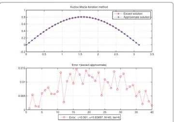
Figure 1 Noise level = 1/100, iter = 5.
Figure 2 Noise level = 1/100, iter = 6.
Figures - show the comparison between the exact solution and its computed approx-imations for different valuesN (:= number of grid points),k(:= number of iterations), ω(:= relaxation factor),ε(:= noisy level) andEr(f) =
fapproximate–fexacte∗
Figure 3 Noise level = 1/1,000, iter = 5.
Table 1 Kozlov-Maz’ya method
N k ω Er(f )
40 5 0.01 0.83697 0.0523 40 6 0.01 0.83697 0.0612 40 5 0.001 0.83697 0.0054 40 6 0.001 0.83697 0.0162
Relative errorEr(f).
6 Conclusion
The numerical results (Figures -, Table ) are quite satisfactory. Even with the noise level ε= ., the numerical solutions are still in good agreement with the exact solution.
In this study, a convergent and stable reconstruction of an unknown initial condition has been obtained using the Kozlov-Maz’ya iteration method. Both theoretical and numerical studies have been provided.
Competing interests
The authors declare that they have no competing interests.
Authors’ contributions
All authors read and approved the final manuscript.
Author details
1Laboratory of Applied Mathematics and Modeling, University 8 Mai 1945 Guelma, P.O. Box 401, Guelma, 24000, Algeria. 2Department of Mathematics, University 8 Mai 1945 Guelma, P.O. Box 401, Guelma, 24000, Algeria.3Applied Mathematics Laboratory, University Badji Mokhtar Annaba, P.O. Box 12, Annaba, 23000, Algeria.
Acknowledgements
This work is supported by the MESRS of Algeria (CNEPRU Project B01120090003).
Received: 8 December 2014 Accepted: 19 March 2015
References
1. Kozlov, VA, Maz’ya, VG: On iterative procedures for solving ill-posed boundary value problems that preserve differential equations. Leningr. Math. J.1, 1207-1228 (1990)
2. Kozlov, VA, Maz’ya, VG, Fomin, AV: An iterative method for solving the Cauchy problem for elliptic equations. USSR Comput. Math. Math. Phys.31(1), 45-52 (1991)
3. Bastay, G: Iterative Methods for Ill-posed Boundary Value Problems. Linköping Studies in Science and Technology, Dissertations No. 392, Linköping University, Linköping (1995)
4. Baumeister, J, Leitao, A: On iterative methods for solving ill-posed problems modeled by partial differential equations. J. Inverse Ill-Posed Probl.9(1), 13-29 (2001)
5. Bouzitouna, A, Boussetila, N: Two regularization methods for a class of inverse boundary value problems of elliptic type. Bound. Value Probl.2013, 178 (2013)
6. Wang, JG, Wei, T: An iterative method for backward time-fractional diffusion problem. Numer. Methods Partial Differ. Equ.30(6), 2029-2041 (2014)
7. Zhang, HW, Wei, T: Two iterative methods for a Cauchy problem of the elliptic equation with variable coefficients in a strip region. Numer. Algorithms65, 875-892 (2014)
8. Atakhadzhaev, MA, Egamberdiev, OM: The Cauchy problem for the abstract bicaloric equation. Sib. Mat. Zh.31(4), 187-191 (1990)
9. Fichera, G: Is the Fourier theory of heat propagation paradoxical? Rend. Circ. Mat. Palermo.41, 5-28 (1992) 10. Joseph, L, Preziosi, DD: Heat waves. Rev. Mod. Phys.61, 41-73 (1989)
11. Fushchich, VL, Galitsyn, AS, Polubinskii, AS: A new mathematical model of heat conduction processes. Ukr. Math. J.42, 210-216 (1990)
12. Ames, KA, Straughan, B: Non-Standard and Improperly Posed Problems. Academic Press, New York (1997) 13. Carasso, AS: Bochner subordination, logarithmic diffusion equations, and blind deconvolution of Hubble space
telescope imagery and other scientific data. SIAM J. Imaging Sci.3(4), 954-980 (2010) 14. Payne, LE: On a proposed model for heat conduction. IMA J. Appl. Math.71, 590-599 (2006)
15. Wang, L, Zhou, X, Wei, X: Heat Conduction: Mathematical Models and Analytical Solutions. Springer, Berlin (2008) 16. Shlapunov, A: On iterations of non-negative operators and their applications to elliptic systems. Math. Nachr.218,
165-174 (2000)
17. Krasnosel’skii, MA, Vainikko, GM, Zabreiko, PP, Rutitskii, YB: Approximate Solutions of Operator Equations. Noordhoff, Groningen (1972)
18. Leiva, H: Controllability of a Generalized Damped Wave Equation. Notas de Matemática, No. 244, Mérida (2006) 19. Pazy, A: Semigroups of Linear Operators and Application to Partial Differential Equations. Springer, Berlin (1983) 20. Fattorini, HO: The Cauchy Problem. Cambridge University Press, Cambridge (1983)