R E S E A R C H
Open Access
An approximate solution of fractional cable
equation by homotopy analysis method
Mustafa Inc
1, Ebru Cavlak
1*and Mustafa Bayram
2*Correspondence:
ebrucavlak@hotmail.com.tr 1Department of Mathematics, Firat
University, Elazı ˘g, 23119, Turkey Full list of author information is available at the end of the article
Abstract
In this article, the homotopy analysis method (HAM) is applied to solve the fractional cable equation by the Riemann-Liouville fractional partial derivative. This method includes an auxiliary parameterhwhich provides a convenient way of adjusting and controlling the convergence region of the series solution. In this study, approximate solutions of the fractional cable equation are obtained by HAM. We also give a convergence theorem for this equation. A suitable value for the auxiliary parameterh is determined and results obtained are presented by tables and figures.
Keywords: cable equation; fractional differential equations; fractional cable equation; homotopy analysis method
1 Introduction
Fractional calculus has a very long history. However, this field lagged behind classic anal-ysis. In fact, the basis of fractional calculus depended on classic analanal-ysis. Especially, in recent years fractional differential equations were used in fluid mechanics, viscoelastic-ity, biology, pharmacy, physics, chemistry and biochemistry, hydrology, medicine, finance, and engineering. The fractional-order models are more useful than integer-order models in many cases. Structures having fractional order are more useful in the studies that have been done by developing technology.
However, the analytic solutions of most fractional differential equations generally can-not be obtained. Thus, fractional differential equations have been solved by many approx-imate methods. Examples are the homotopy perturbation method [, ], the method of separating variables [], the iteration method [], the decomposition method [], and the homotopy analysis method [].
In this study, we will consider the cable equation that has been used in modeling the ion electro diffusion at the neurons. The cable equation occurred due to anomalous dif-fusion and this equation is one of the most fundamental equations for modeling neuronal dynamics []. The cable equation can be derived from the Nernst-Planck equation for electrodiffusion in smooth homogeneous cylinders []. In recent years, studies were con-ducted on various biological and physical systems. In this equation, the diffusion rate of species cannot be characterized by the single parameter of the diffusion constant []. The anomalous diffusion is characterized by a scaling parameterγ as well as the diffusion con-stantDand the mean square displacement of diffusing speciesr(t)scales as a nonlinear
power law in time,i.e., r(t) ∼tγ [–]. Henryet al.derived a fractional cable
equa-tion from the fracequa-tional Nernst-Planck equaequa-tions to model anomalous electrodiffusion of
ions in spiny dentrites []. They subsequently found a fractional cable equation by treating the neuron and its membrane as two separate materials governed by separate fractional Nernst-Planck equations. As a result, the fractional cable equation includes two Riemann-Liouville fractional derivatives.
Consider the following fractional cable equation:
∂u(x,t)
∂t =D
–γ
t
K∂
u(x,t)
∂x
–μD–γ
t u(x,t) +f(x,t), (.)
u(x, ) =g(x), ≤x≤L, (.)
u(,t) =ϕ(t), u(L,t) =ψ(t), ≤t≤T, (.)
where <γ,γ< ,K> andμare constants, andD –γ
t u(x,t) is the Riemann-Liouville fractional partial derivative of order –γ [].
In the literature, there are few treatments of approximate solutions of the fractional cable equation in terms of (.). Equation (.) has been solved by implicit numerical methods (INM) [], the implicit compact difference scheme (ICFDS) [], and explicit numerical methods [].
Here, we will use the HAM, which is an approximate solution to solve this equation. The HAM method was developed in by Liao in []. This method has been successfully applied by many authors [–]. The HAM contains the auxiliary parameterhwhich provides us with a simple way to adjust and control the convergence region of solution series for large or small values ofxandt.
2 Preliminaries and notations
We give some basic definitions and properties of the fractional calculus theory, which are used further in this paper.
Definition . The Euler Gamma function(z) is defined by the so-called Euler integral of the second kind,
(z) =
∞
tz–e–tdt R(z) > , (.)
wheretz–=e(z–)logt. This integral is convergent for all complexz∈/C[].
Definition . The Riemann-Liouville fractional integral operator of orderα≥ of a functionf ∈Cμ,μ≥–, is defined as
D–tαu(x,t) =
(α)
t
(t–τ)α–u(x,τ)dτ, α> ,t> , (.)
and properties of the operatorD–αcan be found in [, ]. Also, some of properties of
operatorD–αare as follows:
(i) D–α
t f(t) =f(t),
(ii) D–xαxγ= (γ + )
(α+γ + )x
α+γ
D–tαtγ= (γ+ )
(α+γ + )t
α+γ
,
(iii) D–tαD–tβf(t) =D
–(α+β)
t f(t),
(iv) D–tαD–tβf(t) =D
–β
t D–tαf(t).
3 Homotopy analysis method
We consider the following differential equation:
Nu(x,t)= , (.)
whereNis a nonlinear differential operator,xandtdenote independent variable;u(x,t) is an unknown function. By means of the HAM, one first constructs a zeroth-order defor-mation equation
( –q)Lφ(x,t;q) –u(x,t)=qhH(t)Nφ(x,t;q), (.)
where q∈[, ] is the embedding parameter, h= is a non-zero auxiliary parameter,
H(t)= is an auxiliary function,Lis an auxiliary linear operator,u(x,t) is an initial guess
ofu(x,t), andφ(x,t;q) is an unknown function. It is important that one has great freedom to choose auxiliary things in the HAM. Obviously, whenq= andq= , we have
φ(x,t; ) =u(x,t), φ(x,t; ) =u(x,t), (.)
respectively. The solutionφ(x,t;q) varies from the initial guessu(x,t) to the solution u(x,t). Expandingφ(x,t;q) in a Taylor series about the embedding parameter, we have
φ(x,t;q) =u(x,t) + ∞
m=
um(x,t)qm, (.)
where
um(x,t) =
m!
∂mφ(x,t;q)
∂qm
q=, m= , , , . . . . (.)
The convergence of the series (.) depends upon the auxiliary parameterh. If it is con-vergent atq= , one has
u(x,t) =u(x,t) +
∞
m=
um(x,t). (.)
According to (.), the governing equation can be deduced from the zeroth-order defor-mation equation (.). Define the vector
un=
u(x,t),u(x,t),u(x,t), . . . ,un(x,t)
.
equa-tion
Lum(x,t) –χmum–(x,t)
=hH(t)Rm(um–,x;t), (.)
where
Rm(um–,x;t) =
(m– )!
∂m–N[φ(x,t;q)]
∂qm–
q=, (.)
and
χm=
, m≤,
, m> . (.)
It should be emphasized thatum(x,t) form≥ is governed by the nonlinear equation (.) with the linear boundary conditions that come from the original problem, which can easily be solved by symbolic computation software such as Maple and Mathematica.
4 Numerical applications and comparison
Consider the following initial and boundary problem of the fractional cable equation:
∂u(x,t)
∂t =D
–γ
t
∂u(x,t)
∂x –D –γ
t u(x,t) +f(x,t), (.)
u(x, ) = , ≤x≤, (.)
u(,t) = , u(,t) = , ≤t≤T, (.)
where f(x,t) = (t+π(+t+γγ) +t(++γγ))sinπx. The exact solution of (.)-(.) isu(x,t) =
tsinπx[].
We choose the linear operator
Lφ(x,t;q)= ∂
∂tφ(x,t;q), (.)
with the propertyL[C] = whereCis a constant. We define a nonlinear operator by
Nφ(x,t,q)=Dtφ(x,t,q) –D–t γ
∂φ(x,t,q)
∂x +D
–γ
t φ(x,t,q) –f(x,t). (.)
Therefore we establish the zeroth-order deformation equation
( –q)Lφ(x,t,q) –u(x,t)=qhH(t)Nφ(x,t,q). (.)
In (.),q= andq= , we can write
φ(x,t, ) =u(x,t), φ(x,t, ) =u(x,t). (.)
So we obtain themth-order deformation equation
Lum(x,t) –χmum–(x,t)
=hH(t)Rm
um–(x,t)
where
Rm
um–(x,t)
=∂um–(x,t)
∂t –D
–γ
t
∂um–(x,t)
∂x +D
–γ
t um–(x,t) –f(x,t) (.)
and
χm=
, m≤,
, m> . (.)
Now the solution of themth-order deformation equation (.) form≥ becomes
um(x,t) =χmum–(x,t) +hH(t)L–
Rm
um–(x,t)
. (.)
Instead ofRm(um–),
um(x,t) =χmum–(x,t) +hH(t)
t
∂um–(x,t)
∂t –D
–γ
t
∂um–(x,t) ∂x
+D–γ
t um–(x,t) –f(x,t)
dt (.)
can be written. The auxiliary functionH(t) can be chosen in the formH(t) = . Rearrangement of (.) gives themth-order deformation equation
um(x,t) =χmum–(x,t) +h
t
Rm
→– um–(x,t)
dt. (.)
Therefore, some of the symbolically computed components are found as
u(x,t) = ,
u(x,t) =htsinπx
– – π
tγ
( +γ)
– t
γ
( +γ)
,
u(x,t) =u(x,t) +h
–tsinπx( + h)πtγ( + γ
)( +γ)
×( +γ+γ)( + γ) +( +γ)
hπtγ( +γ )
×( +γ+γ)( + γ) +· · ·,
u(x,t) =u(x,t) +h
–tsinπx– ht
sinπx–t+γsinπx ( +γ)
–ht
+γsinπx
( +γ)
–h
πt+γ+γsinπx
( +γ+γ)
– hπ
t+γγ ( + γ)( +γ)
+( +γ) ( +γ)
πt+γ(γ ) ( + γ)
sinπx
+ + ht+ ht+γ
πt+γsinπx ( +γ)
+ t
+γsinπx
γ( + γ+γ)
–· · ·, ..
.
As a result, themth-order approximation ofu(x,t) is given by
∞
m=
um(x,t). (.)
Theorem .(Convergence Theorem) As long as the series u(x,t) =u(x,t)+∞m=um(x,t)
converges,where um(x,t)is governed by(.)under the definitions(.)and(.),it must
be a solution of the fractional cable equation(.).
Proof If the series
+∞
m= um(x,t)
converges, then we can write
S(x,t) =
+∞
m= um(x,t)
and we have
lim
n→∞un(x,t) = . (.)
Using definition (.), we get
h ∞
m= Rm
→– um(x,t)
=
∞
m=
Lum(x,t) –χmum–(x,t)
= lim n→∞
∞
m=
Lum(x,t) –χmum–(x,t) =L lim n→∞ ∞ m=
um(x,t) –χmum–(x,t)
=Llim n→∞un(x,t)
= .
Sinceh= ,∞m=Rm(–→um(x,t)) = . From (.), we have
∞
m= Rm
→– um(x,t)
=
∞
m=
Dtum–(x,t) –D– γ
t um–(x,t)xx+D–
γ
t um–(x,t) –F(x,t)
=
∞
m=
Dtum(x,t) –
∞
m= D–γ
t um(x,t)xx+
∞
m= D–γ
t um(x,t) –F(x,t)
=Dt
∞
m=
um(x,t) –D–
γ
t
∞
m=
um(x,t)xx+D–
γ
t
∞
m=
um(x,t) –F(x,t)
=DtS(x,t) –D–t γS(x,t)xx+D–t γS(x,t) –F(x,t)
Table 1 Absolute errors obtained whenγ1=γ2= 0.5,x= 10–4, andh= 1/108
t INM [9] ICFDS [10] HAM
0.1 4.7796×10⁻⁵ 3.4436×10⁻⁶ 3.14159×10⁻⁸
0.2 2.1914×10⁻⁴ 6.8604×10⁻⁶ 6.28319×10⁻⁸
0.3 5.2286×10⁻⁴ 9.8036×10⁻⁶ 9.42478×10⁻⁸
0.4 9.6227×10⁻⁴ 1.2163×10⁻⁵ 1.25664×10⁻⁷
0.5 1.5392×10⁻³ 1.3893×10⁻⁵ 1.5708×10⁻⁷
0.6 2.2552×10⁻³ 1.4974×10⁻⁵ 1.88496×10⁻⁷
0.7 3.1110×10⁻³ 1.5394×10⁻⁵ 2.19911×10⁻⁷ 0.8 4.1015×10⁻³ 1.5141×10⁻⁵ 2.51327×10⁻⁷ 0.9 5.2452×10⁻³ 1.4211×10⁻⁵ 2.82743×10⁻⁷ 1.0 6.5246×10⁻³ 1.2596×10⁻⁵ 3.14159×10⁻⁷
Table 2 Comparison of the HPM, HAM, exact solution (ES) and absolute errors results ofu(x,t) whenγ1=γ2= 0.5,t= 0.1, andh= –0.0395 for 5th-order approximation
x HPM HAM ES Error (HPM) Error (HAM)
0.1 –0.340367 0.00309062 0.00309017 0.343458 4.53322×10⁻⁷
0.2 –0.647417 0.00587871 0.00587785 0.653295 8.6227×10⁻⁷
0.3 –0.891093 0.00809136 0.00809017 0.899184 1.18681×10⁻⁶ 0.4 –1.04754 0.00951196 0.00951057 1.05705 1.39518×10⁻⁶ 0.5 –1.10145 0.0100015 0.01 1.11145 1.46698×10⁻⁶ 0.6 –1.04754 0.00951196 0.00951057 1.05705 1.39518×10⁻⁶ 0.7 –0.891093 0.00809136 0.00809017 0.899184 1.18681×10⁻⁶
0.8 –0.647417 0.00587871 0.00587785 0.653295 8.6227×10⁻⁷
0.9 –0.340367 0.00309062 0.00309017 0.343458 4.53322×10⁻⁷
Table 3 Comparison of the HPM, HAM, exact solution (ES) and absolute errors results ofu(x,t) whenγ1=γ2= 0.25,t= 0.1, andh= –0.004 for 10th-order approximation
x HPM HAM ES Error (HPM) Error (HAM)
0.1 –8614.19 0.00302986 0.00309017 8614.2 6.0306×10⁻⁵ 0.2 –16385.2 0.00576314 0.00587785 16385.2 1.14709×10⁻⁵ 0.3 –22552.2 0.00793229 0.00809017 22552.3 1.57883×10⁻⁴ 0.4 –26511.8 0.00932496 0.00951057 26511.8 1.85603×10⁻⁴
0.5 –27876.1 0.00980485 0.01 27876.1 1.95154×10⁻⁴
0.6 –26511.8 0.00932496 0.00951057 26511.8 1.85603×10⁻⁴
0.7 –22552.2 0.00793229 0.00809017 22552.3 1.57883×10⁻⁴
0.8 –16385.2 0.00576314 0.00587785 16385.2 1.14709×10⁻⁵
0.9 –8614.19 0.00302986 0.00309017 8614.2 6.0306×10⁻⁵
From the initialu(x, ) = andum(x, ) = , we have
S(x, ) =
∞
m=
um(x, ) =u(x,t) +
∞
m=
um–(x, ) = . (.)
Therefore, according to the above expressions,S(x,t) must be the exact solution of (.)
and (.).
We get the following tables and figures by using a series solution obtained with HAM of (.).
5 Conclusion
Table 4 Comparison of the HPM, HAM, exact solution (ES) and absolute errors results ofu(x,t) whenγ1= 0.25,γ2= 0.75,t= 0.1, andh= –0.0043 for 10th-order approximation
x HPM HAM ES Error (HPM) Error (HAM)
0.1 –5022.62 0.00305436 0.00309017 5022.62 3.58117×10⁻⁵ 0.2 –9553.59 0.00580973 0.00587785 9553.6 6.8118×10⁻⁵
0.3 –13149.4 0.00799641 0.00809017 13149.4 9.37564×10⁻⁵
0.4 –15458.0 0.00940035 0.00951057 15458.0 1.10217×10⁻⁴
0.5 –16253.5 0.00988411 0.01 16253.6 1.15889×10⁻⁴
0.6 –15458.0 0.00940035 0.00951057 15458.0 1.10217×10⁻⁴
0.7 –13149.4 0.00799641 0.00809017 13149.4 9.37564×10⁻⁵
0.8 –9553.59 0.00580973 0.00587785 9553.6 6.8118×10⁻⁵
0.9 –5022.62 0.00305436 0.00309017 5022.62 3.58117×10⁻⁵
Figure 1 Thehcurves of 5th-order and 10th-order approximate solutions obtained by the HAM forγ1=γ2= 0.5, respectively.
Figure 2 The 10th-order approximate solution of u(x,t) with different values ofhforγ1=γ2= 0.5 andt= 0.1.
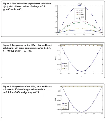
Figure 3 The 10th-order approximate solution of u(x,t) with different values ofhforγ1= 0.8,
γ2= 0.3 andt= 0.5.
Figure 4 Comparison of the HPM, HAM and Exact solution for 5th-order approximate whent= 0.1, h= –0.0395 andγ1=γ2= 0.5.
Figure 5 Comparison of the HPM, HAM and Exact solution for 10th-order approximate when t= 0.1,h= –0.004 andγ1=γ2= 0.25.
The range of convergence control parameterhwas determined by taking a different number of terms of the series solution in Figure . We showed that convergent results can be obtained by selecting the appropriate values ofxandtof the convergence parameter
h= .
An approximate solution that was obtained for different values of the parameterh, the fractional-order derivatives γ, γ of the analytical solution and some comparisons for
some values oftwere presented in Figures -.
A comparison between HPM, HAM, and the analytical solution, whent= . for some values of the auxiliary parameter h= and partial-order derivatives <γ,γ≤, was
made in Figures -. As can be seen from the figures, HAM and the analytical solution coincided and the HPM solution diverged from the analytical solution.
The absolute errors that were obtained by the implicit numerical method [], implicit compact finite difference method [], and HAM can be seen in Table . In this tableγ= γ= . and .≤t≤.. As can be seen from this table when the convergent control
A comparison between HPM, HAM, and the analytical solution forγ,γ and some
values of the auxiliary parameterh= were presented in Tables -. As can be seen from the tables, the HPM solution diverged from the analytical solution but the HAM solution approached the analytical solution.
Although convergent results for almost every value of the independent variables and convergent control parameterhhave been obtained in HAM; the approximate solution diverged at some small and large values of independent variables in HPM. Namely, it is possible to find results that converge rapidly to the analytical solution by HAM.
Consequently HAM is a recommended method for obtaining an approximate solution of the fractional cable equation withγandγRiemann-Liouville derivatives.
Competing interests
The authors declare that they have no competing interests.
Authors’ contributions
All authors contributed equally to the writing of this paper. All authors read and approved the final manuscript.
Author details
1Department of Mathematics, Firat University, Elazı ˘g, 23119, Turkey.2Department of Mathematical Engineering, Yildiz
Technical University, Istanbul, 34220, Turkey.
Received: 25 September 2013 Accepted: 20 February 2014 Published:16 Mar 2014 References
1. Wang, Q: Homotopy perturbation method for fractional KdV equation. Appl. Math. Comput.190, 1795 (2007) 2. Golmakhaneh, AK, Golmakhaneh, AK, Baleanu, D: On nonlinear fractional Klein-Gordon equation. Signal Process.91,
446 (2011)
3. Chen, J, Liu, F, Anh, V: Analytical solution for the time fractional telegraph equation by the method of separating variables. J. Math. Anal. Appl.338, 1364 (2008)
4. Momani, S, Odibat, Z, Alawneh, A: Variational iteration method for solving the space- and time-fractional KdV equation. Numer. Methods Partial Differ. Equ.24(1), 262 (2008)
5. Momani, S: An explicit and numerical solutions of the fractional KdV equation. Math. Comput. Simul.70, 110 (2005) 6. Inc, M: On numerical solution of Burgers’ equation by homotopy analysis method. Phys. Lett. A372, 356 (2008) 7. Langlands, TAM, Henry, B, Wearne, S: Solution of a fractional cable equation: Finite case. Preprint, Submitted to
Elsevier Science http://www.maths.unsw.edu.au/applied/filed/2005/amr05-33.pdf (2005) 8. Keener, J, Sneyd, J: Mathematical Physiology. Springer, Berlin (1991)
9. Liu, F, Yang, Q, Turner, I: Stability and convergence of two new implicit numerical methods for fractional cable equation. In: Proceeding of the ASME 2009 International Design Engineering Technical Conferences & Computers and Information in Engineering Conference, IDETC/CIE, San Diego, California, USA (2009)
10. Hu, X, Zhang, L: Implicit compact difference scheme for the fractional cable equation. Appl. Math. Model.36(9), 4027 (2012)
11. Quintana-Murillo, J, Yuste, SB: An explicit numerical method for the fractional cable equation. Int. J. Differ. Equ. (2011). doi:10.1155/2011/231920
12. Liao, SJ: Beyond Perturbation: Introduction to the Homotopy Analysis Method. Chapman & Hall/CRC, Boca Raton (2003)
13. Inc, M: On exact solution of Laplace equation with Dirichlet and Neumann boundary conditions by the homotopy analysis method. Phys. Lett. A365, 412 (2007)
14. Abbasbandy, S: Soliton solutions for the Fitzhugh-Nagumo equation with the homotopy analysis method. Appl. Math. Model.32, 2706 (2008)
15. Abbasbandy, S, Shivanian, E: Series solution of the system of integro-differential equations. Z. Naturforsch. A64, 811 (2009)
16. Yinping, L, Zhibin, L: The homotopy analysis method for approximating the solution of the modified Korteweg-de Vries equation. Chaos Solitons Fractals39, 1 (2009)
17. Jafari, H, Tajadodi, H, Biswas, A: Homotopy analysis method for solving a couple of evolution equations and comparison with Adomian decomposition method. Waves Random Complex Media21(4), 657-667 (2011) 18. Kilbas, AA, Srivastava, HM, Trujillo, JJ: Theory and Applications of Fractional Differential Equations. North-Holland
Mathematics Studies, vol. 204 (2006)
19. Podlubny, I: Fractional Differential Equations. Academic Press, San Diego (1999) 20. Oldham, KB, Spanier, J: The Fractional Calculus. Academic Press, New York (1974)
10.1186/1687-2770-2014-58
Cite this article as:Inc et al.:An approximate solution of fractional cable equation by homotopy analysis method.