www.astesj.com
Proceedings of International Conference on Applied Mathematics (ICAM’2017), Taza, Morocco
ASTESJournal ISSN:2415-6698
Comparison of K-Means and Fuzzy C-Means Algorithms on
Simplification of 3D Point Cloud Based on Entropy
Estima-tion
Abdelaaziz Mahdaoui∗1, Aziz Bouazi2, Abdallah Marhraoui Hsaini2, El Hassan Sbai2
1Physics Department, Faculty of sciences, Moulay Ismail University, Mekns, Morocco 2Ecole Suprieure de Technologie,Moulay Ismail University, Mekns, Morocco
A R T I C L E I N F O A B S T R A C T Article history:
Received: 13 June, 2017 Accepted: 15 July, 2017 Online: 10 December, 2017
Inthis articlewewillpresentamethod simplifying3Dpointclouds. This method is based on the Shannon entropy. This technique of simplification is a hybrid technique where we use the notion of clustering and iterative computation. In this paper, our main objective isto applyour method ondifferentclouds of3Dpoints. In the clustering phase we will use two different algorithms; K-means and Fuzzy C-means. Then we will make a comparison between the resultsobtained.
Keywords: Simplification 3D
Clustering
1
Introduction
The modern 3D scanners are 3D acquisition tools which are developed in terms of resolution and acqui-sition speed. The clouds of points obtained from the digitization of the real objects can be very dense. This leads to an important data redundancy. This prob-lem must be solved and optimal point cloud must be found. This optimization of the number of points re-sults in reducing the reconstruction calculation.
The problem of simplifying point cloud can be for-malized as follows: given a set of pointsXsampling a surfaceS, find a sample points X0 with|X| ≤ |X|, Such that X0 sampling a surface S0 is close toS. |X|is the cardinality of setX. This objective requires defining a measure of geometric error between the original and simplified surface for which the method will resort to the estimation of the global or local properties of the original surface. There are two main categories of algorithms to sampling points: sub-sampling algo-rithms and resampling algoalgo-rithms. The subsampling algorithms produce simplified sample points which are a subset of the original point cloud, while the re-sampling algorithms rely on estimating the proper-ties of the sampled surface to compute new relevant points.
In the literature, the categories of simplification al-gorithms have been applied according to three main simplification schemes. The first method is simplifi-cation by selection or calculation of points represent-ing subsets of the initial sample. This method consists of decomposing the initial set into small areas, each of which is represented by a single point in the simpli-fied sample [1-4]. The methods of this category are distinguished by the criteria defining the areas and their construction.
The second method is iterative simplification. The principle of iterative simplification is to remove points of the initial sample incrementally per geomet-ric or topologic criteria locally measuring the redun-dancy of the data [5-10].
The third method is simplification by incremen-tal sampling. Unlike iterative simplification, the sim-plified sample points can be constructed by progres-sively enriching an initial subset of points or sampling an implicit surface [11-18].
This paper will present a hybrid simplification technique based on the entropy estimation [19] and clustering algorithm [20].
It is organized as follows: In section 2, we will re-call some density function estimators. In section 3, we will present clustering algorithm. Then in section 1∗
Corresponding Author: Abddelaaziz Mahdaoui, Email: [email protected]
4, we will present our 3D point cloud simplification algorithm based on Shannon entropy [21]. Section 5 will show the results and validation. Finally, we will present the conclusion.
2
Defining the Estimation of
Den-sity Function and Entropy
There are several methods for density estimation: parametric and nonparametric methods. We will fcus on nonparametric methods which include the kernel density estimator, also known as the Parzen-Rosenblatt method [22,23] and the K nearest neigh-bors (K-NN) method [24]. We will only use in this ar-ticle K-NN estimator.
2.1
The K Nearest Neighbors Estimator
The algorithm of the k nearest neighbors (K-NN) [24] is a method of estimating the nonparametric probabil-ity of the densprobabil-ity function. The degree of estimation is defined by an integer k which is the number of the nearest neighbors, generally proportional to the size of the sample N. For each x we define the estimation of the density. The distances between points of the sample and x are as follows:
r1(x)< ... < rk−1(x)< rk(x)< ... < rN(x)
riwith (i= 1...k...N) are distances sorted by ascending
order.
The estimator k-NN in dimensiondcan be defined as follows:
pknn(x) = k N
Vk(x)
=
k N
Cdrk(x)
(1)
whererk(x) is the distance fromxto the kth
near-est point andVk(x) is the volume of a sphere of radius.
rk(x) andCd is the volume of the unit sphere in d
di-mension.
The numberk must be adjusted as a function of the sizeN of the available sample in order to respect the constraints that ensure the convergence of the estima-tor. For N observations, the k can be calculated as follows:
k=k0
√ N
By respecting these rules of adjustment, it is cer-tain that the estimator converges when the numberN increases indefinitely whatever is the value ofk0.
2.2
Defining Entropy
Claude Shannon introduced the concept of the en-tropy which is associated with a discrete random vari-ableX as a basic concept in information theory [21]. The distribution of probabilitiesp =p1, p2, ..., pN
as-sociated with the realizations ofX. The Shannon en-tropy is calculated by using the following formula:
H(p) =−
N
X
i=1
p(xi) log(p(xi)) (2)
Entropy measures the uncertainty associated with a random variable. Therefore, the realization of the rare event provides more information about the phe-nomenon than the realization of the frequent event.
3
Clustering Algorithms
Defini-tion
X = {xi ∈ Rd}, i = 1, , N is a set of observations de-scribed by d attributes; the objective of clustering is the structuring of data into homogeneous classes. Clustering is unsupervised classification. The objec-tive is to try to group clustered points or classes so that the data in a cluster is as similar as possible. Two types of approaches are possible; hierarchical and non-hierarchical approaches[25].
In this article, we will concentrate on the non-hierarchical approach which is encapsulated in both the Fuzzy C-Means Clustering (FCM) algorithm [26,20] and K-means algorithm (KM)[27].
3.1
Fuzzy C-Means Clustering Algorithm
Fuzzy c-means is a data clustering technique wherein each data point belongs to a cluster to some degree that is specified by a membership grade. This tech-nique was originally introduced by J.C. Dunn[20], and improved by J.C. Bezdek[26] as an improvement on earlier clustering methods. It provides a method that shows how to group data points that populate some multidimensional space into a specific number of dif-ferent clusters.
X={x1, x2, ..., xn}is a given data set to be analysed, andV ={v1, v2, ..., vc} is the set of centers of clusters in X data set in p dimensional space Rp. Where N is the number of objects,pis the number of features andcis the number of partitions or clusters. FCM is a clustering method allowing each data point to belong to multiple clusters with varying degrees of member-ship.
FCM is based on the minimization of the following objective function
Jm= c
X
i=1
N
X
j=1
uijmDijA2 (3)
Where, DijA2 is the distances betweenith features vector and the centroid ofjth cluster. They are com-puted as a squared inner-product distance norm in Equation (4):
DijA=kxj−vik= (xj−vi)TA(xj−vi) (4)
In the objective function in Equation (3),U is a fuzzy partition matrix that is computed from data setX:
U=uij (5)
overlap refers to how fuzzy the boundaries between clusters are. That is the number of data points that have significant membership in more than one clus-ter.
The objective function is minimized with the con-straints as follows: uij ∈ [0,1]; 1 ≤ i ≤ c; 1 ≤ j ≤
N; Pc
i=1uij= 1; 0<PNi=1uij< N;
FCM performs the following steps during cluster-ing:
1. Randomly initialize the cluster membership values,uij.
2. Calculate the cluster centres:
PN
i=1umijxj
PN
i=1uijm
.
3. Updateuij according to the following:
1
PN
k=1(DijA/DkjA)2/(m−1)
4. Calculate the objective function,Jm
5. Compare U(t+1) withU(t), where t is the itera-tion number.
6. IfkU(t+1)−U(t)k< εthen it stop, or else returns to the step 2. (ε is a specified minimum thresh-old, in this case it usesε= 10−5).
3.2
K-Means Clustering Algorithm
The K-Means algorithm (KM) iteratively computes the cluster centroids for each distance measurement in or-der to minimize the sum with respect to the specified measure. The objective of the K-Means algorithm is to minimize an objective function named by squared error function given in equation (6) as follows:
Jkm(X;V) = c
X
i=1
N
X
j=1
Dij2 (6)
Dij2 is the chosen distance measure which is in Eu-clidean norm:kxij−vik2, 1≤i≤c,1≤j≤Ni. Where Ni represents the number of data points inithcluster.
Forc clusters, the K-Means algorithm is based on an iterative algorithm that minimizes the sum of the dis-tances of each object at its cluster center. The goal is to have a minimum value of the sum of the distance by moving the objects between the clusters. The steps of K-means are as follows:
1. Centroids of c clusters are chosen from X ran-domly.
2. Distances between data points and cluster cen-troids are calculated.
3. Each data point is assigned to the cluster whose centroid is close to it.
4. Cluster centroids are updated by using the for-mula in Equation (7):
vi= Ni
X
i=1
xij
Ni
(7)
5. Distances from the updated cluster centroids are recalculated.
6. If no data point is assigned to a new cluster, the execution of algorithm is stopped, otherwise the steps from 3 to 5 are repeated taking into con-sideration probable movements of data points between the clusters.
4
Evaulation of the Simplified
Meshes
In order to give a theoretical evaluation for the simpli-fication method, we have based on a metric of mean errors, max error and RMS(root mean square error) used by Cignoni et al.[28]. Where he measured the Hausdorff distance between the approximation and the original model. Hausdorff distance is defined as follow:
Let X and Y be two non-empty subsets of a metric space (M, d). We define their Hausdorffdistance
dH=max{sup x∈X
inf
y∈Y
(d(x, y), sup
y∈Y
inf
x∈X
(d(x, y))} (8)
In our experiments we will use the symmetric Hausdorff distance calculated with the Metro soft-ware tool[28].
In order to calculate the approximate error, we will re-construct the models from the point clouds. We find in the literature several reconstruction techniques [29] to create a 3D model from a set of points.
5
Proposed Approach
Now, we will propose an algorithm to simplify dense 3D point cloud. First, this algorithm is based on the entropy estimation algorithm. It allows the estima-tion of the entropy for each 3D point ofXas well as making the decision to eliminate or to keep the point. In this pproach we will use the K-NN estimator to es-timate the entropy. Moreover, it is based on clustering algorithm (KM or FCM) to subdivide point cloudX into clusters in order to minimize the computation time. The procedures are:
SIMPLIFICATION ALGORITHM
• Input
– X ={x1, x2, , xN} : The data simple (point cloud)
– S: threshold
– c: the number of clusters
• Begin
• Decomposing the initial set of points X into c small areas denotingRj(j= 1,2, ..., c), and using
clustering algorithm (FCM or KMA).
• Forj= 1 toc
– Calculate global entropy of a cluster j by using all data samples in Rj ={y1, y2, , ym}
according to the equation (2), Note this en-tropyH(Rj).
– Calculate the entropy H(Rj−yi) of point
cloudRjless pointyi(i= 1,2, , m)
– Calculate 4Hi =| H(Rj)−H(Rj−yi)| with i= 1,2, , m
– If4Hi ≤SThen Rj=Rj−yi.
– End-if
• End for End.
6
Results and Discussion
To validate the efficiency of the use of the two clus-tering algorithms FCM and KM in our simplifica-tion method, we use three 3D models that represent real objects such as Max Planck (fig. 1,b) and Atene (fig. 1,a). Fig. (2,a), (2,b) show simplification re-sults on various point cloud using FCM algorithm. Fig. (3,a), (3,b) show simplification results on various point cloud using KM algorithm.
(a) (b)
Figure 1:original point cloud, a) Atene, b) Max Planck
(a) (b)
Figure 2:Simplified point cloud using FCM algorithm, a) Atene, b) Max Planck
(a) (b)
Figure 3: Simplified point cloud using KM algorithm, a) Atene, b) Max Planck
(a)
(b)
(c)
(a)
(b)
(c)
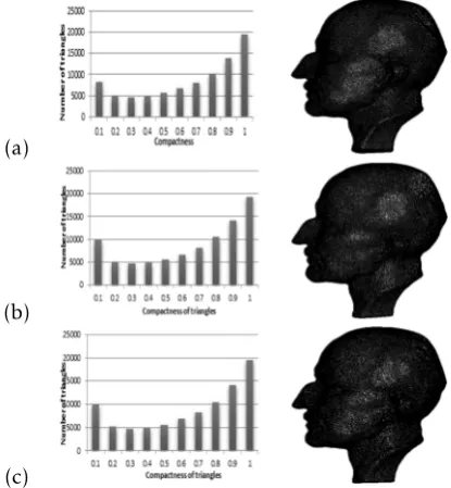
Figure 5: Comparison of Atene mesh quality, a) Original point cloud, b) simplified point cloud using FCM, c) simplified point cloud using KM
In this section, we will validate the effectiveness of our proposed method. Actually, we have conducted a comparison between the original and simplified point cloud. Accordingly, we will use a comparison between the original and simplified mesh.
Thereafter, we make a comparison between the original mesh and the one created from the simpli-fied point cloud. To reconstruct the mesh, we use ball Pivoting method [31,29] or A.M Hsaini et al. method [32]. Then, to measure the quality of the obtained meshes, we compute the quality of the triangles using the compactness formula proposed by Guziec [33]:
c= 4 √
3a
l12+l22+l32 (9)
Whereli are the lengths of the edges of the triangle.
Anda is the area of the triangle. We note that this measure is equal to 1 for an equilateral triangle and 0 for a triangle whose vertices are collinear. According to [34], a triangle is an acceptable quality ifc≥0.6.
In figures 4, 5, we have presented the trian-gles compactness histogram of the two meshes. In each figure, the first line presents the reconstructed mesh from the original point cloud. The second line presents the simplified point cloud using FCM algo-rithm. The third line presents the simplified point cloud using KM algorithm. Note that, the evaluation of the mesh quality is achieved by the compactness of the triangles.
Depending on [34] meshes are compact if the per-centage of the number of triangles, which composes mesh with compactnessc≥0.6 is greater than or equal to 50%. Also, according to the histograms in figures 4 and 5, it is observed that the surfaces obtained from the simplified point cloud are compact surfaces.
The table 1 also shows that the use of the KM and
FCM algorithms retains the compactness of the sur-faces. However, the compactness obtained by the FCM algorithm is greater than that obtained by KM for the two surfaces.
Concerning the number of vertices obtained after simplification, we note that this number is higher in the case of FCM for the two models.
It is interesting to note that in the case where FCM is used better results are produced in terms of speed. In contrast, in the other case where KM is used the speed is slow.
Table 3 and table 4 shows the numerical results ob-tained by the implementation of the two algorithms FCM and KM in the simplification method. The main results are average error, maximal error and root mean square error (RMS).
Figure 6 and 7 present differences between origi-nal and simplified meshes using Hausdorff distance. Note that it is a red-green-blue map, so red is min-imal and blue is maxmin-imal, so in our case red means zero error and blue high error.
a) b)
Figure 6: difference between original and simplified MaxPlanck mesh
a) b)
Figure 7:difference between original and simplified Atene mesh
Table 3 presents the results relative to the eval-uation of the approximation error concerning Max-Planck model. Table 4 Also presents the same error related to Atene model.
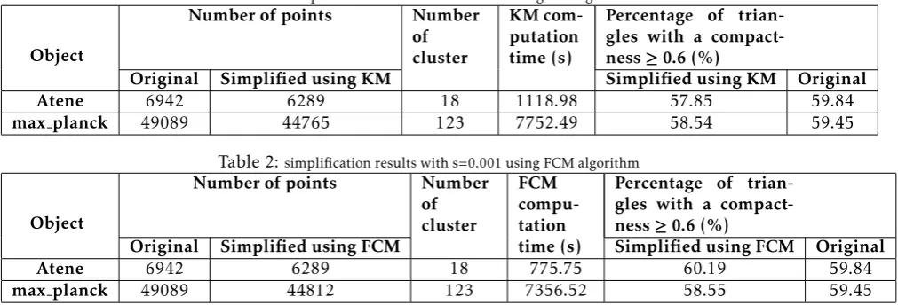
Table 1: simplification results with s=0.001 using KM algorithm
Object
Number of points Number
of cluster
KM com-putation time (s)
Percentage of trian-gles with a compact-ness≥0.6 (%)
Original Simplified using KM Simplified using KM Original
Atene 6942 6289 18 1118.98 57.85 59.84
max planck 49089 44765 123 7752.49 58.54 59.45
Table 2:simplification results with s=0.001 using FCM algorithm
Object
Number of points Number
of cluster
FCM compu-tation time (s)
Percentage of trian-gles with a compact-ness≥0.6 (%)
Original Simplified using FCM Simplified using FCM Original
Atene 6942 6289 18 775.75 60.19 59.84
max planck 49089 44812 123 7356.52 58.55 59.45
Table 3:Comparison of FCM and KM algorithm used in simplification method: MaxPlanck mesh (errors are measured as percentages of the datasets bounding box diagonal (699.092499))
Methods Number of vertex Number of faces (triangles) Average Error Max Error RMS Error
Entropy-KM 44765 89355 0.000010 0.001799 0.000054
Entropy-FCM 44567 88960 0.000010 0.002241 0.000055
Table 4:Comparison of FCM and KM algorithm used in simplification method: Atene mesh (errors are measured as percentages of the datasets bounding box diagonal (6437.052937))
Methods Number of vertex Number of faces (triangles) Average Error Max Error RMS Error
Entropy-KM 6289 11746 0.000153 0.016014 0.000697
Entropy-FCM 6446 9543 0.000331 0.016022 0.000930
shown figures 6.a et figure 7.a. By contrast, it is in-teresting to note that this method produces the best results when speed is needed (look at table 2).
As expected, KM algorithm in table 1 yields good results in terms of average error, max error and RMS error. Moreover, she recorded in general the worst re-sult in terms of calculation speed.
We have implemented our simplification method under MATLAB. The calculations are performed on a machine with an i3 CPU, 3.4 Ghz, with 2GB of RAM.
7
Conclusion
This work presents a brief overview of two cluster-ing algorithms, K-means and C-means. The results of an empirical comparison are presented to make a comparison between the use of the clustering algo-rithms. These clustering algorithms are integrated in our method of simplifying 3D point clouds. We have compared the computation time and the precision of the simplified meshes.
From the point of view of accuracy, the results show that K-means gives the best results in terms of error. As for claculation time, the use of Fuzzy C-means algorithm makes simplification faster.
8
Acknowledgment
The Max Planck and Atene models used in this paper are the courtesy of AIM@SHAPE shape repository.
References
1. M. Pauly, M. Gross, and L. P. Kobbelt, Efficient simplification of point-sampled surfaces, in IEEE Visualization, 2002. VIS 2002., pp. 163170.
2. J. Wu and L. Kobbelt, Optimized Sub-Sampling of Point Sets for Surface Splatting, Comput. Graph. Forum, vol. 23, no. 3, pp. 643652, Sep. 2004.
3. Y. Ohtake, A. Belyaev, and H.-P. Seidel, An integrating ap-proach to meshing scattered point data, in Proceedings of the 2005 ACM symposium on Solid and physical modeling -SPM 05, 2005, pp. 6169.
4. B.-Q. Shi, J. Liang, and Q. Liu, Adaptive simplification of point cloud using K-means clustering, Comput. Des., vol. 43, no. 8, pp. 910922, Aug. 2011.
5. L. Linsen, Point cloud representation, Univ. Karlsruhe, Ger. Tech. Report, Fac. Informatics, pp. 118, 2001.
6. T. K. Dey, T. K. Dey, J. Giesen, and J. Hudson, Decimating Samples for Mesh Simplification, in PROC. 13TH CANA-DIAN CONF. COMPUT. GEOM, 2001, pp. 85–88.
7. N. Amenta, S. Choi, T. K. Dey, and N. Leekha, A simple algo-rithm for homeomorphic surface reconstruction, in Proceed-ings of the sixteenth annual symposium on Computational geometry - SCG 00, 2000, pp. 213222.
8. M. Alexa, J. Behr, D. Cohen-Or, S. Fleishman, D. Levin, and C. T. Silva, Point set surfaces, in Proceedings Visualization, 2001. VIS 01., 2001, pp. 2128.
9. M. Garland and P. S. Heckbert, Surface simplification us-ing quadric error metrics, in Proceedus-ings of the 24th an-nual conference on Computer graphics and interactive tech-niques - SIGGRAPH 97, 1997, pp. 209216.
10. R. Allegre, R. Chaine, and S. Akkouche, Convection-driven dynamic surface reconstruction, in International Conference on Shape Modeling and Applications 2005 (SMI 05), pp. 3342.
12. Boissonnat J. D. and S. Oudot, Provably good surface sam-pling and approximation, in Proceedings of the 2003 Eu-rographics/ACM SIGGRAPH symposium on Geometry pro-cessing, 2003, pp. 918.
13. J.-D. Boissonnat and S. Oudot, An effective condition for sampling surfaces with guarantees, in Proceedings of the ninth ACM symposium on Solid modeling and applications, 2004, pp. 101112.
14. J.-D. Boissonnat and S. Oudot, Provably good sampling and meshing of surfaces, Graph. Models, vol. 67, no. 5, pp. 405451, Sep. 2005.
15. L. P. Chew and L. Paul, Guaranteed-quality mesh genera-tion for curved surfaces, in Proceedings of the ninth annual symposium on Computational geometry - SCG 93, 1993, pp. 274280.
16. A. Adamson and M. Alexa, Approximating and Intersecting Surfaces from Points, in In Proc. Symposium on Geometry Processing, 2003, pp. 230239.
17. M. Pauly and M. Gross, Spectral processing of point-sampled geometry, in Proceedings of the 28th annual conference on Computer graphics and interactive techniques - SIGGRAPH 01, 2001, pp. 379386.
18. A. P. Witkin and P. S. Heckbert, Using particles to sample and control implicit surfaces, in Proceedings of the 21st an-nual conference on Computer graphics and interactive tech-niques - SIGGRAPH 94, 1994, pp. 269277.
19. Jing Wang, Xiaoling Li, and Jianhong Ni, Probability density function estimation based on representative data samples, in IET International Conference on Communication Tech-nology and Application (ICCTA 2011), 2011, pp. 694698. 20. J. C. Dunn, A Fuzzy Relative of the ISODATA Process and
Its Use in Detecting Compact Well-Separated Clusters, J. Cy-bern., vol. 3, no. 3, pp. 3257, Jan. 1973.
21. C. E. Shannon, A mathematical theory of communication, ACM SIGMOBILE Mob. Comput. Commun. Rev., vol. 5, no. 1, p. 3, Jan. 2001.
22. E. Parzen, On Estimation of a Probability Density Function and Mode, Ann. Math. Stat., vol. 33, pp. 10651076.
23. M. Rosenblatt, Remarks On Some Nonparametric Estimates of a Density Function, Ann. Math. Stat., vol. 27, no. 3, pp. 832837, Sep. 1956.
24. B. W. Silverman, Density estimation for statistics and data analysis. Chapman and Hall, 1986.
25. A. K. Jain, Data clustering: 50 years beyond K-means, Pat-tern Recognit. Lett., vol. 31, no. 8, pp. 651666, Jun. 2010.
26. J. C. Bezdek, Pattern Recognition with Fuzzy Objective Function Algorithms. Boston, MA: Springer US, 1981.
27. G. Gan and M. K.-P. Ng, k -means clustering with outlier re-moval, Pattern Recognit. Lett., vol. 90, pp. 814, Apr. 2017.
28. P. Cignoni, C. Rocchini, and R. Scopigno, Metro: Measuring Error on Simplified Surfaces, Comput. Graph. Forum, vol. 17, no. 2, pp. 167174, Jun. 1998.
29. A. Mahdaoui, A. Marhraoui Hsaini, A. Bouazi, and E. H. Sbai, Comparative Study of Combinatorial 3D Reconstruc-tion Algorithms, Int. J. Eng. Trends Technol., vol. 48, no. 5, pp. 247251, 2017.
30. H.-G. Mller and A. Petersen, Density Estimation Including Examples, in Wiley StatsRef: Statistics Reference Online, Chichester, UK: John Wiley and Sons, Ltd, 2016, pp. 112.
31. F. Bernardini, J. Mittleman, H. Rushmeier, C. Silva, and G. Taubin, The ball-pivoting algorithm for surface reconstruc-tion, IEEE Trans. Vis. Comput. Graph., vol. 5, no. 4, pp. 349359, Oct. 1999.
32. A. M. Hsaini, A. Bouazi, A. Mahdaoui, E. H. Sbai, and A. R. Bernstein-bezier, Reconstruction and adjustment of surfaces from a 3-D point cloud, nternational J. Comput. Trends Technol., vol. 37, no. 2, pp. 105109, 2016.
33. A. Gueziec and Andr, Locally toleranced surface simplifica-tion, IEEE Trans. Vis. Comput. Graph., vol. 5, no. 2, pp. 168189, 1999.