M. Ismail, B. Maury & J.-F. Gerbeau, Editors
FLUID-PARTICLES FLOWS: A THIN SPRAY MODEL WITH ENERGY
EXCHANGES
Laurent Boudin
1,2, Benjamin Boutin
1,3, Bruno Fornet
4, Thierry Goudon
5,6,
Pauline Lafitte
5,6, Fr´
ed´
eric Lagouti`
ere
5,7and Benoˆıt Merlet
8Abstract. This paper is devoted to an asymptotic analysis of a fluid-particles coupled model, in the bubbling regime. On the theoretical point of view, we extend the analysis done in [4] for the case of an isentropic gas to the case of an ideal gas, thus adding the internal energy, or temperature, which is unknown. We formally derive the bubbling limit system in the same way as in [4] and propose a numerical scheme to solve this limit system.
The numerical resolution of the non-limit system, and the numerical analysis of the asymptotic properties of the scheme (e.g. the asymptotic preserving property), as performed in [4], is at study.
R´esum´e. Nous proposons ici une analyse asymptotique formelle d’un mod`ele de couplage entre une densit´e de particules et un fluide, dans la limite ditebubbling. Cette analyse est effectu´ee en suivant les pas de [4] o`u le fluide consid´er´e est isentropique tandis qu’il est ici un gaz parfait (o`u donc l’´energie interne, ou la temp´erature, est une inconnue suppl´ementaire). Nous identifions le syst`eme limite et proposons un algorithme pour le r´esoudre de mani`ere approch´ee.
La suite de ce travail, en cours, concerne l’´ecriture d’un algorithme de r´esolution du syst`eme non limite, et l’´etude des propri´et´es asymptotiques dudit sch´ema.
1.
Introduction
We are interested in a PDE system describing the interaction between a fluid and a set of droplets immersed in the fluid. This situation occurs in combustion theory [15], motivated for instance by the design of engines or propulsors [11]. We also mention the dynamics of sprays with many applications e.g. biomedical sprays [2], dispersion of pollutants [13], the optimization of fine water spray fire suppression systems... The fluid is described by the evolution of its density ρ(t, x) ≥ 0, its velocity u(t, x) ∈ RN (N = 1, 2 or 3) and its total energy
1
UPMC Paris 06, Lab. J.-L. Lions, 175 rue du Chevaleret, BC 187, F-75013 Paris, France; e-mail:[email protected] & [email protected]
2
INRIA Paris-Rocquencourt, REO Project team, BP 105, F-78153 Le Chesnay Cedex, France.
3
CEA, DEN/DANS/DM2S/SFME/LETR, F-91191 Gif-sur-Yvette, France.
4
DTIM/ONERA Centre de Toulouse, 2 avenue Edouard Belin, 31055 Toulouse, France. e-mail:[email protected] 5
Project-Team SIMPAF, INRIA Lille Nord Europe Research Centre Park Plazza, 40 avenue Halley 59650 Villeneuve d’Ascq CEDEX, France; e-mail:[email protected] & [email protected]
Laboratoire Paul Painlev´e, USTL-CNRS UMR 8524, Cit´e Scientifique, 59655 Villeneuve d’Ascq CEDEX, France.
7
Universit´e Paris Diderot-Paris 7, Lab. J.-L. Lions, 175 rue du Chevaleret, BC 187, F-75013 Paris, France.
8
Universit´e Paris Nord - Institut Galil´ee LAGA (Laboratoire d’Analyse, G´eom´etrie et Applications) Avenue J.B. Cl´ement 93430 Villetaneuse, France; e-mail:[email protected]
c
E(t, x) ≥ 0, which are functions of time t ≥ 0 and position x ∈ RN. We define the internal energy e, the pressurep, the temperature Θ by the relations
e= p
(γ−1)ρ ≥0, p=RρΘ, E=e+ u2
2
where R is the perfect gas constant and γ >1 is the adiabatic constant. The disperse phase is described by its density distribution in phase spacef(t, x, v)≥0, where the variable v ∈RN stands for the velocity of the particles. Macroscopic quantities can be defined as moments with respect tov; in what follows we need
the macroscopic density: n(t, x) =
Z
RN
f(t, x, v) dv,
the bulk velocity: nV(t, x) =
Z
RN
v f(t, x, v) dv,
the temperature: n|V|2(t, x) +N nΘ
p=
Z
RN|
v|2 f(t, x, v) dv,
the heat flux: q(t, x) =
Z
RN
v |v|
2
2 f(t, x, v) dv.
The evolution of the densityf is governed by
∂tf+v· ∇xf = divv (v−u)f + Θ∇vf)−ηp∇xΦ· ∇vf. (1)
The divergence term in the right-hand side accounts for both the friction force exerted by the fluid on the particles, which is supposed to be proportional to the relative velocity (v −u), and the Brownian motion of the particles, which induces diffusion with respect to the velocity variable, depending on the surrounding temperature Θ. Note that more complicated and nonlinear expressions of the drag force can be used; the linear relation with respect to the relative velocity applies when the Reynolds number of the flow is low. The second term in the right-hand side comes from an external force with potential Φ and ηp is a positive constant. The
evolution of the fluid obeys the Euler system
∂tρ+ divx(ρu) = 0,
∂t(ρu) + Divx(ρu⊗u) +∇xp=F −ηfρ∇xΦ,
∂t(ρE) + divx (ρE+p)u) =E −ηfρu· ∇xΦ,
(2)
whereηf is another positive coefficient that accounts for a possible difference of amplitude in the forces applied
to the fluid or the disperse phase. Remark that assuming ηp and ηf positive means that the external force
associated to the potential Φ acts on opposite directions on the particles and on the fluid. Bearing in mind the example of gravity we have ∇xΦ =g ∈RN and we are dealing with a situation where particles are light
compared to the fluid: gravity pushes the fluid downward, while buoyancy effects push the particles upward. In other words, here and below, the disperse phase is buoyancy driven, while the fluid is gravity driven. In such a situation, we can expect the formation of sedimentation profiles. We refer to [3], [4] for a discussion on this modeling issue. Here, the main point we address is the introduction of the energy equation and the description of energy exchanges.
In (2), the force F arising in the right-hand side of the momentum equation is given by the friction force exerted by the particles on the fluid and it reads
F(t, x) =n(V −u)(t, x) = Z
RN
The energy exchanges between the two phases split as follows:
E(t, x) = n(V −u)·u+N n(Θp−Θ)(t, x) +E′(t, x)
=
Z
RN
(v−u)f(t, x, v) dv·u
+N(Θp−Θ)(t, x)
Z
RN
f(t, x, v) dv+E′(t, x).
(4)
In this expression, the first term is nothing but the work of the friction forceF while the second describes the heat transfer between the two phases; the last term, which will be specified later on, guarantees the total energy conservation. As a matter of fact, we remark that the evolution of the internal energy is driven by
∂t(ρe) + divx(ρeu) +pdivxu=N n(Θp−Θ) +E′(t, x).
In this modeling, we disregard many physical effects that could be non negligible for applications (added mass effects, Basset forces...). Nevertheless in most cases, these effects are of many orders smaller than the drag and gravity forces. We restrict ourselves to the description of thin sprays which means that
- we neglect inter-particles collisions and coagulation-fragmentation phenomena. - the volume fraction of the particles is neglected as well.
We refer for instance to [12] for further discussions of the modeling issues.
In this paper, the goal is to extend, at least formally, the analysis performed in [3] (see also [9, 10]) and, having identified relevant asymptotic regimes, to design adapted Asymptotic Preserving schemes, in the spirit of [4, 5, 8]. The dissipative or relaxation properties of the system are crucial to this approach.
2.
Dissipation properties
Let us start by considering the evolution of the macroscopic quantities
∂tn+ divx(nV) = 0,
∂t(nV) + Divx
Z
RN
v⊗vf dv=−n(V −u) +ηpn∇xΦ,
∂t
Z
RN
v2 2 f dv
+ divxq=−
Z
RN
(v−u)·v f dv+N nΘ +ηpnV · ∇xΦ,
(5)
where we use integration by parts for evaluating the right-hand sides. Observe that the total momentum is conserved (up to the gravity term) since
∂t(ρu+nV) + Divx
ρu⊗u+
Z
RN
v⊗vf dv+∇xp= (ηpn−ηfρ)∇xΦ. (6)
Next, since we consider the mixture fluid/particles as a whole, the total energy should also be conserved, which will give the definition ofE′. We remark that
Z
RN
(v−u)·v f dv =
Z
RN|
v−u|2f dv+n(V −u)·u
= n(|V|2+NΘ
p−2V ·u+|u|2) +n(V −u)·u
= n|V −u|2+N nΘp+n(V −u)·u.
Therefore the kinetic energy of the particles obeys
∂t
Z
RN |v|2
2 f dv
Accordingly, we set
E′(t, x) =n|V −u|2
so that the total energy is driven by
∂t
ρE+
Z
RN |v|2
2 f dv
+ divx (ρE+p)u+q= (ηpnV −ηfρu)· ∇xΦ. (7)
Hence, the term E′ appears as a source of internal energy, or a source of heat, for the fluid, produced by the friction with the particle, and proportional to the macroscopic kinetic energy defined by the relative velocity
V −u.
Next, we consider the entropyS(t, x) defined by the relation
S=−γR
−1ln pρ −γ
=−γR −1ln
R Θ ργ−1
.
We check that it satisfies
∂t(ρS) + divx(ρSu) =
Rρ
p n(V −u)·u−n(V −u)·u−N n(Θp−Θ)−E
′
= −N nΘp
Θ −1
−Θn|V −u|2.
(8)
Finally, we look at the entropy of the disperse phase
d dt
Z
RN Z
RN
fln(f) dv dx = − Z
RN Z
RN
(v−u)f· ∇fvf + Θ|∇vf| 2
f
dv dx
= N
Z
RN
ndx− Z
RN Z
RN
Θ|∇vf| 2
f dv dx.
Hence, the total entropy satisfies
d dt
Z
RN
ρSdx+
Z
RN Z
RN
fln(f) dv dx
=− Z
RN Z
RN
Θ|∇vf| 2
f dvdx+ 2N
Z
RN
ndx
−N
Z
RN
nΘp
Θ dx−
Z
RN
n|V −u|2 Θ dx
The next argument is two-fold. On the one hand, we observe that
N
Z
RN
ndx=− Z
RN Z
RN
v−V
√
Θ
p
f·√Θ∇√vf
f dv dx,
and on the other hand we have
Z
RN|
It follows that d dt
Z
RN
ρSdx+
Z
RN Z
RN
fln(f) dv dx
=− Z RN Z RN
Θ|∇vf| 2
f + 2 v−V
√
Θ
p
f ·√Θ∇√vf
f +
|v−V|2 Θ f
dv dx
− Z
RN
n|V −u|
2
Θ dx =− Z RN Z RN √
Θ∇√vf
f + v−V
√ Θ p f 2
dv dx− Z
RN
n|V −u|
2
Θ dx,
which indicates that the total entropy of the system is dissipated. Let us summarize the computation as follows.
Proposition 1. Let(ρ, u, E, f)be a (smooth enough) solution of (1)–(4). Then, both the total momentum and the total energy are conserved while the total entropy is dissipated and we have
d dt
Z
RN
ρE dx+
Z
RN Z
RN
v2
2 f dv dx
=
Z
RN
(ηpnV −ηfρu)· ∇xΦ dx,
d dt
Z
RN
ρS dx+
Z
RN Z
RN
fln(f) dv dx
=− Z RN Z RN √
Θ∇√vf
f + v−V
√ Θ p f 2
dv dx− Z
RN Z
RN
f|V −u|
2
Θ dv dx≤0.
(9)
Note that the dissipation terms vanish when
u=V and f(t, x, v) = n(t, x)
2πΘ(t, x)N/2 exp
−|v−V(t, x)| 2
2Θ(t, x)
.
3.
Bubbling Regime
According to [3], the “Bubbling Regime” relies on the following scaling:
∂tfǫ+
1
ǫv· ∇xf
ǫ= 1
ǫ2divv (v−ǫu
ǫ)fǫ+ Θǫ∇ vfǫ)−
1
ǫ∇xΦ· ∇vf
ǫ,
∂tρǫ+ divx(ρǫuǫ) = 0,
∂t(ρǫuǫ) + Divx(ρǫuǫ⊗uǫ) +∇xpǫ=1
ǫ
Z
RN
(v−ǫuǫ)fǫ dv−1 1 −ǫ2ρ
ǫ
∇xΦ,
∂t(ρǫEǫ) + divx (ρǫEǫ+pǫ)uǫ)
= 1
ǫ2 Z
RN
(v−ǫuǫ)fǫdv·ǫuǫ+N nǫ(Θǫp−Θǫ) +nǫ|Vǫ−ǫuǫ|2
−1 1
−ǫ2ρ
ǫuǫ
· ∇xΦ,
(10)
where it is convenient to introduce the following notation
nǫ=
Z
RN
fǫ dv, Jǫ= 1
ǫn
ǫVǫ=Z
RN
v ǫ f
ǫ dv,
nǫ|Vǫ|2+N nǫΘǫ p=
Z
RN
v2 fǫdv, qǫ=Z
RN
v ǫ
v2 2 f
ǫ dv.
The scaling can be explained as follows. Given the radius d of the particles, the particles densityρp and the
typical fluid densityρf, the dynamic viscosity of the fluid µwe define the Stokes settling time
τS =
2ρpd2
and the Stokes settling velocity
VS =τSg|1−ρf/ρp|.
Dropping a particle in the fluid at rest,VS is the asymptotic velocity of the particle, andτS the corresponding
relaxation time. Hence, τS characterizes the strength of the drag force andVS characterizes the effect of the
external force, here gravity-buoyancy, on the particles. Then, we introduce time and length scales of observation,
T and L respectively and we setU =L/T which stands for the velocity unit. It is the typical velocity of the fluid. It has to be compared to bothVS and the thermal velocity
Vth=
s
3kΘ 4πρpd3,
with Θ a typical value of the temperature and k the Boltzmann constant. The scaling assumes the following relations
τS =ǫ2T ≪T, VS ≃U =ǫVth, ρp=ǫρf.
Therefore, the Richardson number, which is the ratio of potential to kinetic energy, is 1/(1−ǫ2) for the fluid and 1/ǫfor the particles. Similarly, the temperature relaxation is characterized by
τth=
1
N u4πdΛΘ
where N u is the Nusselt number, and Λ the thermal conductivity. We remind that the Nusselt number is a dimensionless ratio of convection heat transfer to fluid conduction heat transfer. In the present context, we have the following relation
τth=ǫ2T.
Of course, many other different scaling are relevant, as described in the above mentioned references. Never-theless, we restrict ourselves to this regime, extension of the bubbling regime considered in [3, 4]. Our goal is two-fold:
- firstly, we derive the asymptotic hydrodynamic system corresponding to the limitǫ→0,
- secondly, we design a numerical scheme for the limit system and comment on numerics the influence of the energy exchanges.
In this context Proposition 1 recasts as
d dt
Z
RN
ρǫEǫ dx+
Z
RN Z
RN
v2 2 f
ǫ dv dx=Z
RN nǫVǫ
ǫ − ρǫuǫ
1−ǫ2
· ∇xΦ dx,
d dt
Z
RN
ρǫSǫ dx+
Z
RN Z
RN
fǫln(fǫ) dv dx
+1
ǫ2 Z
RN Z
RN h
√
Θǫ∇vf ǫ
√
fǫ +
v−Vǫ
√
Θǫ
p
fǫ 2
+fǫ|Vǫ−ǫuǫ|2idv dx≤0,
(11)
and we infer the following relaxation effects
Vǫ≃ǫuǫ
fǫ(t, x, v)≃ nǫ(t, x)
2πΘǫ(t, x)N/2 exp
−|v−V
ǫ(t, x)|2 2Θǫ(t, x)
≃nǫ(t, x)MΘǫ(t,x)(v)
whereMΘ stands for the centered Maxwellian with temperature Θ
MΘ(v) = (2πΘ)−N/2 e−v
2/(2Θ)
Accordingly, we obtain
Z
RN
v2fǫ dv=nǫ|Vǫ|2+N nǫΘǫ p≃
Z
RN
v2 nǫM
Θǫ dv=N nǫΘǫ
withVǫ expected to be of orderO(ǫ). We deduce that
Θǫ−Θǫ p−−−→
ǫ→0 0
(an observation which can be seen also by considering the energy equation). Eventually, we guess that the asymptotic behavior is described by the evolution of the macroscopic quantitiesn, ρ, u,Θ only, and we assume that
(nǫ, ρǫ, uǫ,Θǫ)−−−→
ǫ→0 (n, ρ, u,Θ) (in a strong enough sense...), and consequently
fǫ(t, x, v)→n(t, x)MΘ(t,x)(v). (12)
It thus remains to determine the equations satisfied by these quantities.
To this end, we go back to the moments equations (5) which recast here in the following rescaled form
∂tnǫ+ divx(Jǫ) = 0,
ǫ2∂
tJǫ+ Divx
Z
RN
v⊗vfǫ dv=−Jǫ+nǫuǫ+nǫ∇xΦ,
∂t
Z
RN
v2 2 f
ǫdv+ div xqǫ=
1 ǫ2 − Z RN
(v−ǫuǫ)·v fǫ dv+N nǫΘǫ−1ǫ∇x·
Z
RN |v|2
2 ∇vf
ǫ dv
= 1
ǫ2 n
ǫ(−|Vǫ|2−NΘǫ
p+ǫuǫ·Vǫ+NΘǫ
+n
ǫVǫ
ǫ · ∇xΦ
=N nǫ Θ ǫ−Θǫ
p
ǫ2 +J
ǫ·uǫ−Jǫ
nǫ +∇xΦ
.
(13)
We also suppose that
(Jǫ, qǫ)−−−→ǫ
→0 (J, q)
holds and we wish to relate these limits to (n, ρ, u,Θ). The ansatz (12) allows to compute the limit of the second moment Z
RN
v⊗v fǫ dv−−−→
ǫ→0 n Z
RN
v⊗v MΘ(v) dv=nΘI.
Therefore, lettingǫgo to 0 in the momentum equation leads to
0 +∇x(nΘ) =−J+n(u+∇xΦ). (14)
Next, we consider the equation for the total energy
∂t
ρǫEǫ+
Z
RN |v|2
2 f
ǫ dv+ div
x (ρǫEǫ+pǫ)uǫ+qǫ= (Jǫ−
ρǫuǫ
1−ǫ2)· ∇xΦ. (15)
Asǫ→0 we get
∂t
ρE+N 2nΘ
+ divx (ρE+p)u+q= (J −ρu)· ∇xΦ. (16)
We are left with the task of identifying the heat flux q. To this purpose, we observe that
ǫ2∂tqǫ+Divx
Z
RN
v⊗v|v|
2
2 f
ǫdv=
−3qǫ+
Z
RN
v⊗v+|v| 2
2 I
fǫdvuǫ+(N+2)ΘǫJǫ− Z
RN
v|v|
2
Hence, whenǫgoes to 0 we find
0 +∇x
n
2N
Z
RN|
v|4MΘ(v) dv
=∇x
N+ 2
2 nΘ 2
= N+ 2 2 Θ
2
∇xn+ (N+ 2)nΘ∇xΘ
=−3q+N+ 2
2 nΘ(u+∇xΦ) + (N + 2)Θ n(u+∇xΦ)− ∇x(nΘ)
=−3q+3
2(N+ 2)nΘ(u+∇xΦ)−(N + 2)(nΘ∇xΘ + Θ 2∇
xn).
sinceR
RN|v| 4M
1(v) dv=N(N+ 2). It defines the heat fluxqby means ofn, u and Θ:
q= N+ 2
2 nΘ(u+∇xΦ)−
N+ 2 2 Θ
2 ∇xn−
2(N+ 2)
3 nΘ∇xΘ. The conclusion of the computations states as follows.
Theorem 1. Assuming strong enough convergence of the macroscopic quantities, the limit as ǫ goes to 0 is described by the following set of PDEs
∂tρ+ divx(ρu) = 0,
∂tn+ divx nu− ∇x(nΘ)=−divx(n∇xΦ),
∂t(ρu) + Divx(ρu⊗u+p) =−∇x(nΘ) + (n−ρ)∇xΦ,
∂t
ρE+N 2 nΘ
+ divx
(ρE+p)u+N+ 2 2 nΘu
= N+ 2 2 divx(Θ
2∇
xn) +
2(N+ 2)
3 divx(nΘ∇xΘ)
−N2+ 2divx(nΘ∇xΦ) + (n−ρ)u∇xΦ +n|∇xΦ|2− ∇xΦ· ∇x(nΘ).
(17)
In System (17) the unknowns are the fluid densityρ, the particle (macroscopic) densitynand the common velocityuand temperature Θ. Assuming a constant temperature and dropping the energy equation, we recover the equations derived in [3]. There appear some unusual terms in the equations which are reminiscent of the so-called Soret and Dufour effects, see [14]. The Soret effect relies on the conduction currentn∇xΘ: the
temperature gradient produces a flow of particles. Note that particles are also subject to diffusion with a diffusion coefficient proportional to the temperature. The Dufour effect relies on the effects of concentration gradients on the evolution of the temperature.
Another way of deriving the limit equations consists in considering fluctuations in the ansatz (12). This approach motivates the design of “Asymptotic Preserving” schemes, see [4, 5, 8]. Namely, we set
fǫ(t, x, v) =nǫ(t, x)MΘǫ(t,x)(v) +ǫrǫ(t, x, v)
and we wish to identify the limitrof (rǫ) by using the equation
ǫ∂tfǫ+v· ∇xfǫ=LΘǫrǫ−uǫ· ∇vfǫ− ∇xΦ· ∇vfǫ (18)
whereLΘstands for the Fokker-Planck operator
LΘf = divv(vf+ Θ∇vf)
(recall that LΘ(MΘ) = 0 for every Θ∈R). Indeed, assuming thatrǫ converges tor, we can express the mass and heat fluxes as follows
Jǫ=
Z
RN
vrǫ dv−−−→ǫ
→0 J = Z
RN
vr dv, qǫ=
Z
RN
v|v|
2
2 r
ǫdv
−−−→ǫ
→0 q= Z
RN
v|v|
2
In the the last two terms of (18), the leading contribution reads
−(uǫ+∇xΦ)· ∇v(nǫMΘǫ) = +(uǫ+∇xΦ)· v
Θǫn ǫM
Θǫ.
Therefore,ris characterized by the relation
LΘr = v· ∇x(nMΘ)−(u+∇xΦ)· v ΘnMΘ = vMΘ·
∇xn−(u+∇xΦ)
n
Θ−
N
2
n
Θ∇xΘ
+v|v|
2
2 MΘ·
n
Θ2∇xΘ.
(19)
The solution splits as follows
r=r1+r2,
r1(t, x, v) =χ(t, x, v)·∇
xn−(u+∇xΦ)
n
Θ−
N
2
n
Θ∇xΘ
,
r2(t, x, v) =λ(t, x, v)· n Θ2∇xΘ,
where χ= (χ1, ..., χN) and λ= (λ1, ..., λN) are solutions of the auxiliary problems (wheret, x appear only as
parameters through the temperature)
LΘ(t,x)χj =vjMΘ(t,x), LΘ(t,x)λj=vj |v| 2
2 MΘ(t,x).
We check readily that
χ=−vMΘ, λ=−vMΘ 1 3
|v|2
2 + (N+ 2)Θ
.
The associated mass fluxes are given by
Jχ =
Z
RN
v⊗χdv=− Z
RN
v⊗vMΘdv=−ΘI,
Jλ =
Z
RN
v⊗λdv=− Z
RN
v⊗v1
3
v2
2 + (N + 2)Θ
MΘ dv
= −13(N+ 2) (1/2 + 1) Θ2I=−N2+ 2 Θ2I,
while for the heat flux we obtain
qχ=
Z
RN
vv
2
2 ⊗χdv=−
N+ 2 2 Θ
2 I,
qλ=
Z
RN
vv
2
2 ⊗λdv=− 1 3
(N+ 4)(N+ 2)
4 +
(N+ 2)2 2
Θ3I.
Finally, we are led to the following asymptotic behavior
Jǫ−−−→ ǫ→0 Jχ·
∇xn−(u+∇xΦ)
n
Θ−
N
2
n
Θ∇xΘ
+Jλ·
n
Θ2∇xΘ, =−Θ∇xn+n(u+∇xΦ) +
N
2n∇xΘ−
Similarly, we obtain
qǫ−−−→ ǫ→0 qχ·
∇xn−(u+∇xΦ)
n
Θ−
N
2
n
Θ∇xΘ
+qλ·
n
Θ2∇xΘ =−N+ 2
2
Θ2∇
xn−nΘ(u+∇xΦ)−
N
2 nΘ∇xΘ
−(N+ 4)(N+ 2) + 2(N+ 2) 2
12 nΘ∇xΘ =N+ 2
2 nΘ(u+∇xΦ)−
N+ 2 2 Θ
2∇
xn−
2(N+ 2)
3 nΘ∇xΘ.
We summarize the result as follows.
Proposition 2. The fluctuationrǫ converges to
r=−vMΘ·
∇xn−(u+∇xΦ)
n
Θ−
N
2
n
Θ∇xΘ
−vMΘ
1 3
v2
2 + (N+ 2)Θ
· n
Θ2∇xΘ,
and the mass and heat fluxes have the following behavior
J =n(u+∇xΦ)− ∇x(nΘ),
q= N+ 2
2 nΘ(u+∇xΦ)−
N+ 2 2 Θ
2 ∇xn−
2(N+ 2)
3 nΘ∇xΘ.
It allows to identify the limit in (13), and, of course, we recover in this way System (17).
4.
Numerical scheme for the limit system
In the section we explore the limit system (17) from a numerical point of view. The space dimension isN = 1 in the following, and the potential is gravitational: ∇xΦ =g; System (17) reads
∂tρ+∂x(ρu) = 0,
∂tn+∂x nu=∂x,x2 nΘ
−g∂x(n),
∂t(ρu) +∂x(ρu⊗u+p) =−∂x(nΘ) + (n−ρ)g,
∂t
ρE+N 2nΘ
+∂x
(ρE+p)u+3 2nΘu
=3 2∂x(Θ
2∂
xn) + 2∂x(nΘ∂xΘ)−
5
2g∂x(nΘ) + (n−ρ)ug+ng 2.
The numerical scheme that we derived is based on the following form of the system: denoting ˜p=p+nΘ and
ρE˜ =ρE+nΘ/2, the system can be recast as
∂tρ+∂x(ρu) = 0,
∂tn+∂x nu=∂x,x2 nΘ
−g∂x(n),
∂t(ρu) +∂x(ρu⊗u+ ˜p) = (n−ρ)g,
∂t
ρE˜+∂x
(ρE˜+ ˜p)u
=3 2∂x(Θ
2∂
xn) + 2∂x(nΘ∂xΘ)−
5
2g∂x(nΘ) + (n−ρ)ug+ng 2.
• The first stage solves the system without the right-hand side above:
∂tρ+∂x(ρu) = 0,
∂tn+∂x nu= 0,
∂t(ρu) +∂x(ρu⊗u+ ˜p) = 0,
∂t
ρE˜+∂x
(ρE˜+ ˜p)u= 0.
Here we note the similarity with the classical Euler system. For this stage a standard Lagrange-remap scheme, as in [6], [7], is used. The stability of this stage relies on a hyperbolic-type condition on the time step: the time step of the whole time iteration is determined by this “hyperbolic” condition.
• The second stage solves the dissipative terms as well as the “transport” terms due to the gravity:
∂tρ= 0,
∂tn=∂x,x2 nΘ
−g∂x(n),
∂t(ρu) = 0,
∂t
ρE˜=3 2∂x(Θ
2∂
xn) + 2∂x(nΘ∂xΘ)−5
2g∂x(nΘ).
This stage imposes a parabolic-type stability condition on the time step and is sub-cycled in the time step.
• the last stage solves the gravity terms:
∂tρ= 0,
∂tn= 0,
∂t(ρu) = (n−ρ)g,
∂t
ρE˜= (n−ρ)ug+ng2.
This is done numerically with an explicit Euler scheme.
5.
Numerical results
The space domain is a bounded interval (namely [0,4] in the following) and the chosen boundary conditions are wall boundary conditions: concerning the fluid,u= 0 and∂xp= 0. The boundary condition to be imposed
on Θ is to be derived from the microscopic equations. The wall condition on the microscopic densityf reads
f(t, x, v) =f(t, x,−v) for everyv∈R, whenxbelongs to the boundary. From (19) we have thatrobeys
LΘr=vMΘ∂xn−(u+g)n Θ−
1 2
n
Θ∂xΘ +
v2n 2Θ2∂xΘ
.
We remark that, imposing thatris an even function in thevvariable on the boundary, the left-hand side is an even function and the right-hand side is an odd function. Thus one has
∂xn−(u+g)
n
Θ− 1 2
n
Θ∂xΘ +
v2n
2Θ2∂xΘ = 0,
for everyv ∈R. Thus∂xΘ = 0 and ∂xn= (u+g)n/Θ =gn/Θ on the boundary.
The first numerical result we propose is the case of an isentropic fluid with pressure lawp=ργ(γ≥1, namely
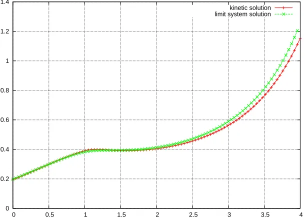
final time isT = 2. On figures 1,2,3 we observe the strong similarity between the two numerical solutions. This similarity is improved when refining the mesh and havingǫdecrease.
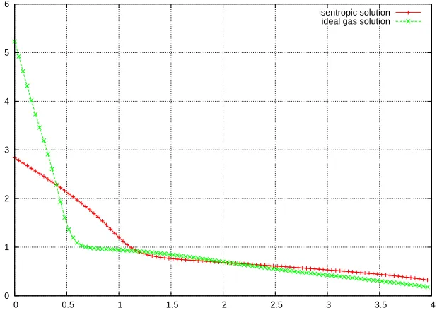
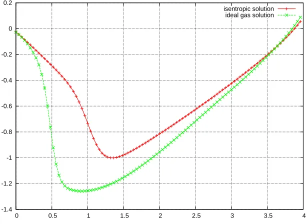
The second series of numerical results are obtained with the same initial conditions, but we want here to analyze the effect of temperature. We thus compare the results of the limit system for an isentropic gas and for an ideal gas. On this first and preliminary result, we see that the thermal effect is not negligible. Figure 7 shows that the temperature has strong variations in the space variable. The consequences concerning the fluid density are particularly important, inducing a high fluid density region on the left-hand side (which can be considered as the bottom, since gravity makes the fluid go leftwards) of the domain. There is a lot of energy on the left-hand side, because of the fluid ”falling down” with a high velocity, as we can see in Figures 4, 6 and 7. On the right-hand side, on the contrary, since the particles are going rightwards slowly because of the buoyancy effect, there is very little energy.
References
[1] C. Baranger, G. Baudin, L. Boudin, B. Despr´es, F. Lagouti`ere, E. Lap´ebie and T. Takahashi. Liquid jet generation and break-up. InNumerical Methods for Hyperbolic and Kinetic Equations, S. Cordier, Th. Goudon, M. Gutnic, E. Sonnendr¨ucker Eds., IRMA Lectures in Mathematics and Theoretical Physics, vol. 7, EMS Publ. House, 2005.
[2] C. Baranger, L. Boudin, P.-E. Jabin and S. Mancini. A modeling of biospray for the upper airways.ESAIM:Proc, 14:41–47, 2005.
[3] J.-A. Carrillo and Th. Goudon. Stability and asymptotics analysis of a fluid-particles interaction model.Comm. PDE, 31:1349– 1379, 2006.
[4] J.-A. Carrillo, Th. Goudon and P. Lafitte. Simulation of Fluid & Particles Flows: Asymptotic Preserving Schemes for Bubbling and Flowing Regimes.J. Comput. Phys., 227(16):7929-7951, 2008.
[5] J.-A. Carrillo, Th. Goudon, P. Lafitte, and F. Vecil. Numerical schemes of diffusion asymptotics and moment closures for kinetic equations.J. Sci. Comput., 36(1):113-149,2008.
[6] B. Despr´es, In´egalit´e entropique pour un solveur conservatif du syst`eme de la dynamique des gaz en coordonn´ees de Lagrange. C. R. Acad. Sci. Paris S´er. I Math. 324 (1997) no 11, p. 1301–1306.
[7] G. Gallice, Sch´emas de type Godunov entropiques et positifs pr´eservant les discontinuit´es de contact. C. R. Acad. Sci. Paris S´er. I Math. 331 (2000) no 2, p. 149–152.
[8] Th. Goudon, P. Lafitte. Splitting schemes for the simulation of non equilibrium radiative flows.Preprint, 2007.
[9] Th. Goudon, P.-E. Jabin and A. Vasseur. Hydrodynamic limit for the Vlasov-Navier-Stokes equations. I. Light particles regime.
Indiana Univ. Math. J., 53(6):1495–1515, 2004.
[10] Th. Goudon, P.-E. Jabin and A. Vasseur. Hydrodynamic limit for the Vlasov-Navier-Stokes equations. II. Fine particles regime.
Indiana Univ. Math. J., 53(6):1517–1536, 2004.
[11] M. Massot and Ph. Villedieu. Mod´elisation multi-fluide eul´erienne pour la simulation de brouillards denses polydispers´es.C. R. Acad. Sci. Paris S´er. I Math., 332(9):869–874, 2001.
[12] J. Mathiaud. Etude de syst`emes de type gaz-particules. PhD thesis, ENS Cachan, Sept. 2006.
[13] B. Sportisse. Mod´elisation et simulation de la pollution atmosph´erique. Habilitation `a Diriger les Recherches, Sciences de l’Univers, Universit´e Pierre et Marie Curie, June 2007.
0 0.5 1 1.5 2 2.5 3
0 0.5 1 1.5 2 2.5 3 3.5 4
kinetic solution limit system solution
Figure 1. Fluid density: comparison of the limit solution and the solution with ǫ= 0.1.
0 0.2 0.4 0.6 0.8 1 1.2 1.4
0 0.5 1 1.5 2 2.5 3 3.5 4
kinetic solution limit system solution
0 0.2 0.4 0.6 0.8 1 1.2 1.4
0 0.5 1 1.5 2 2.5 3 3.5 4
kinetic solution limit system solution
Figure 3. Fluid velocity: comparison of the limit solution and the solution withǫ= 0.1.
0 1 2 3 4 5 6
0 0.5 1 1.5 2 2.5 3 3.5 4
isentropic solution ideal gas solution
0 0.2 0.4 0.6 0.8 1 1.2 1.4
0 0.5 1 1.5 2 2.5 3 3.5 4
isentropic solution ideal gas solution
Figure 5. Particles macroscopic density: comparison of the isentropic and the ideal gas solutions.
-1.4 -1.2 -1 -0.8 -0.6 -0.4 -0.2 0 0.2
0 0.5 1 1.5 2 2.5 3 3.5 4
isentropic solution ideal gas solution
1.2 1.3 1.4 1.5 1.6 1.7 1.8 1.9 2 2.1
0 0.5 1 1.5 2 2.5 3 3.5 4
ideal gas solution