423
Available online at http://ijdea.srbiau.ac.ir
Int. J. Data Envelopment Analysis (ISSN 2345-458X)
Vol.2, No.3, Year 2014 Article ID IJDEA-00232,7 pagesResearch Article
Resource Allocation through Context-dependent
data envelopment analysis
N. Ebrahimkhani Ghazia*, M. Ahadzadeh Naminb,
(a) Department of Mathematics, Science and Research Branch, Islamic Azad University, Tehran, Iran.
(b) Department of Mathematics, Shahr-e –Qods Branch, Islamic Azad University, Tehran, Iran.
Received 8 March 2014, Revised 15 June 2014, Accepted 14 August 2014
Abstract
System designs, optimizing resource allocation to organization units, is still being considered as a complicated problem especially when there are multiple inputs and outputs related to a unit. The algorithm presented here will divide the frontiers obtained with DEA. In this way, we investigate a new approach for resource allocation.
Keywords: DEA, context-dependent, budget allocation, cost-efficiency, efficiency
.
1. Introduction
Our literature review indicates that to this day in the evaluation of decision making units (DMUs) all
DEA models have been used: many models are given only the amounts of inputs and outputs, each
DMU corresponding to the considered inputs and outputs selects its best set of weights; the values of
weights vary from one DMU to another. Each DMU’s performance score is calculated by the DEA
models which range between zero and one that provides its relative degree of efficiency. Moreover, the
sources and amounts of inefficiency in each input and output for every DMU are also identified through
the models. The subject of debate here is the possibility of further exploiting of available data to develop
DEA-type models which help DMUs design their optimal systems and not just evaluate their existing
systems.
* Corresponding author: [email protected]
N. Ebrahimkhani Ghazi ,et al /IJDEA Vol.2, No.3, (2014).423-429 424
In fact, the purpose of this paper is to show the kind of budget allocations to DMUs as a result of which
we have maximum revenue and minimum cost. Budget allocation is the distribution and division of
services and facilities among people and existing programs. In this process, the allocation is done
through Context-dependent data envelopment analysis [4]. In each level we calculate respective X Y
and find the frontier which if budget B is allocated to DMUs in this level, maximum revenue and
minimum cost will be resulted.
1. Discussion and summery
1.1. Determining Levels
Assume that DMUj (j=1… n) produces the outputs Yj (y ,..., y )1j sj by consuming
j 1j mj
X (x ,..., x )the inputs [3]. And also suppose that Jl{DMU ; j 1,..., n}j is all DMUs set. We
define l 1 l l
J J E that Ej{DMU ; Jj l1 *(l, k) 1} and *(l, k)is the optimal solution value for the following linear programming problem:
j L
L
*
j j k
j F( J )
j j k
j F( J )
L j
, (l, k )
(l, k)
Max
(l, k)
s.t.
x
x
y
(l, k)y ;
0,
j
F(J ).
Where(x , y )k k present input and output vector with respect toDMUk, respectively. jF(J )L shows that
l j
DMU J , F(.) proposed a correspondence between a set of DMUs and the analogue common indices
set.
Model (1) is an output oriented CCR [5], where L=1 and defines DMUs which are in the first level
efficiency frontier. DMUs which are in Elset define Lth-efficient level. When L=2 the model (1), after
removing DMUs in the first level, gives us DMUs in the second efficient level.
In this method, multiple efficient levels are recognized. These efficient levels will be obtained by the
following algorithm:
Step1: set L=1, assess all the DMUs set, l
J , through the model (1) DMUs which are efficient in the first
level can be reached.
Step2: Leave out DMUs that are considered in step1. l 1 l l
J J E (Stop when l 1
J )
Step3: Consider a new subset of inefficient DMUs through the model (1) we gain a new set of efficient
DMUsEl 1 (The new efficient frontier.)
Step4: Let L=L+1. Go to step2.
Stopping rule: l 1
J , the algorithm stops.
1.2. Measuring profit efficiency
Now we consider profit efficiency model that helps to optimize DMUs system design. Let’s suppose
DMU (x,y) present benchmark DMU that with inputs T
1 2 m
X(x , x ,..., x ) 0corresponding with cost
T
1 2 m
C(c , c ,..., c ) 0 and output vector T
1 2 s
Y(y , y ,..., y ) 0 corresponding with prices
T
1 2 s
P(p , p ,..., p ) 0. Note that both input vector x and output vector y are now variables. The
calculation of maximum attainable profit, within the DEA framework, is the starting point of a profit
analysis which can be done by using the model shown in [4]:
Where
P
r andw
i are, respectively, the price of rth output and cost of it h inputj
DMU , and the rest
of the notation is as previously defined. Model (2) assures us to reach maximization profit value.
s m
r r i i
r 1 i 1
n
j ij i
j 1
n
j rj r
j 1
n
j ij io
j 1
n
j rj ro
j 1
n
j j
j 1
Max P y C x
s. t . x x , i 1,..., m;
y y , r 1,..., s
x x , i 1,..., m;
y y , r 1,..., s
1; 0, j 1,..., n
N. Ebrahimkhani Ghazi ,et al /IJDEA Vol.2, No.3, (2014).423-429 424
Therefore, for different weights (
P
r,w
i), different price and cost is possible. So Profit efficiency of oDMU
is:s m
r ro i io
r 1 i 1
s m
* *
r r i i
r 1 i 1
P y C x
PE
P y C x
;
2. Budget Allocation through Context-dependent DEA
One of the main activities of management is making a strategy that is possible to deploy. In
organizations that the strategic management has not been implemented resource allocation is based on
politics and personal factors. In strategic oriented organizations resource is allocated on the basis of the
preferences which are determined through the annual purposes.
Budget provides the possibility of allocating the limited resources based on planning preferences. One
of the big barriers is the unsuccessful connection between administrative programs and specifying
priorities regarding allocating budget to enduring guideline programs.
The model mentioned above, implicitly could make the information of budget resource portfolio
available for DMUs, such as an optimum budget and budget congestion.
In this section the purpose is to introduce an algorithm which helps us to fairly allocate the total available
budget B among DMUs. For comparison, the allocation is done by Context-dependent DEA method.
Supposing that the total budget B is available we follow this algorithm:
Step1: Find the efficient level as mentioned in section 2.1. Let these efficient level’s names
1 2 L
E , E ,..., E .
Step2: In each level, distinctly calculate (x,y) in model (2). (For more information see section 2.2 and
Fig 3.1) Suppose the profit value for each level;E , E ,..., E1 2 L, respectively, is 1, 2,...,L.
Step3: For finding the percentage allocation of budget B in each efficient level this indices will be used:
j
j L
j j 1
B
; j 1,..., L
(3),
Which 1 2 n 1 2 n
L L L L L L
j j j j j j
j 1 j 1 j 1 j 1 j 1 j 1
B B B
... B( ... ) B
j
is the allocation rate of constant budget B to DMUs in efficient level
E
jas if constant budget B is fairly allocated to all DMUs.Table 2.Input-data for the 20 bank branches.
j
DMU x1j x2 j x3 j
1 5007.37 36.29 87243
2 2926.81 18.8 9945
3 8732.7 25.74 47575
4 945.93 20.81 19292
5 8487.07 14.16 3428
6 13759.35 19.46 13929
7 587.69 27.29 27827
8 4646.39 24.52 9070
9 1554.29 20.47 412036
10 17528.31 14.84 8638
11 2444.34 20.42 500
12 7303.27 22.87 16148
13 9852.15 18.47 17163
14 4540.75 22.83 17918
15 3039.58 39.32 51582
16 6585.81 25.57 20975
17 4209.18 27.59 41960
18 1015.52 13.63 18641
19 5800.38 27.12 19500
20 1445.68 28.96 31700
Table 1.Inputs and outputs.
Inputs Outputs
Payable interest The total sum of four main deposits Personnel Other deposits
Non-performing loans
Loans granted Received interest Fee
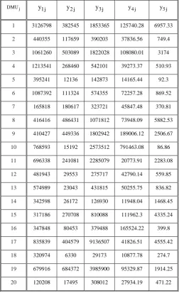
Table 3.Output-data for the 20 bank branches.
j
DMU y1j y2 j y3 j y4 j y5 j
1 3126798 382545 1853365 125740.28 6957.33
2 440355 117659 390203 37836.56 749.4
3 1061260 503089 1822028 108080.01 3174
4 1213541 268460 542101 39273.37 510.93
5 395241 12136 142873 14165.44 92.3
6 1087392 111324 574355 72257.28 869.52
7 165818 180617 323721 45847.48 370.81
8 416416 486431 1071812 73948.09 5882.53
9 410427 449336 1802942 189006.12 2506.67
10 768593 15192 2573512 791463.08 86.86
11 696338 241081 2285079 20773.91 2283.08
12 481943 29553 275717 42790.14 559.85
13 574989 23043 431815 50255.75 836.82
14 342598 26172 126930 11948.04 1468.45
15 317186 270708 810088 111962.3 4335.24
16 347848 80453 379488 165524.22 399.8
17 835839 404579 9136507 41826.51 4555.42
18 320974 6330 29173 10877.78 274.7
19 679916 684372 3985900 95329.87 1914.25
20 120208 17495 308012 27934.19 471.22
Fig. 3.1.levels and revenue efficiency value
N. Ebrahimkhani Ghazi ,et al /IJDEA Vol.2, No.3, (2014).423-429 424
3. Application
Now we will consider the branches of one of the Iran’s commercial banks with 3 inputs and 5 outputs
(see Table2 and Table3) as our DMUs. The inputs are payable interest, personnel and non-performing
loans and the outputs are the total sum of four main deposits, other deposits, loans granted, received
interest and fee (see table1). These data were collected in 2005. First based on the algorithm in section
2.1 we find three levels:
Level1 = {1,4,6,7,8,9,10,11,15,17,19}
Level2 = {2, 3, 5, 14, 16, 18, 20}
Level3 = {12, 13}
Consider the data given in Table 1 and Table 2. Let B = 1,000,000, C = (4, 2, 5) and P = (6, 7, 5, 4, 8).
The unified model (2) is a linear program and thus can be solved by any LP algorithm. So we have:
Profit efficiency in first frontier is: 29,075,477.720000
Profit efficiency in second frontier is: 2,334,938.880000
Profit efficiency in third frontier is: 5,888,766.984000
As shown above the first frontier has the maximum revenue and minimum cost value but logically it is
not a good way to allocate all the budget to the first level because DM wants to have fair judgment in
the society. Not only the main aim of DM is having fair distribution of budget so that all the DMUs
have a sufficient resource but also ensures that the maximum profit will satisfy DM.
We contribute 3 levels in allocation in this way:
1, 000, 000 29, 075, 477.720000 1, 000, 000 29, 075, 477.720000
29, 075, 477.720000 2, 334, 938.880000 5,888, 766.984000 37, 299,183.584 779, 520
1, 000, 000 2, 334, 938.880000 1, 000, 000 2, 334, 938.880000
29, 075, 477.720000 2, 334, 938.880000 5,888, 766.984000 37, 299,183.584 62, 600
1, 000, 000 5,888, 766.984000 1, 000, 000 5,888, 766.984000
29, 075, 477.720000 2, 334, 938.880000 5,888, 766.984000 37, 299,183.584 157,880
It means that the best way to allocate budget in this example is giving 779,520 of budget B to the first
4. Conclusion
We can use the above approach, wherever there is a human need, to allocate a limited budget to a
number of teams or some of the activities so that the case which is chosen from a variety of combinations
of allocations will have the most output value. Applying the optimization models allows all the various
allocation cases to be considered and the most optimized of them which is based on objective function
to be selected. The presented algorithm will enable us to allocate the limited budget to all DMUs. This
was properly examined in a case study in an Iranian bank. Although obviously the first frontier has the
largest proportion of budget, the rest of levels are fairly allocated.
References
[1] Andersen, P., Petersen, N.C., (1993). A procedure for ranking efficient units in data envelopment
analysis. Management Science 39, 1261–1264.
[2] Charnes A, Cooper WW, Rhodes E, (1978) Measuring the efficiency of decision making units.
European Journal of Operational Research; 2:429–44.
[3] Cooper, W. W., Seiford, L. M., & Tone, K. (2007). Data envelopment analysis: A comprehensive
text with models, application, references and DEA-solver software.
[4] Fare, R., S. Grosskopf and C.A. K. Lovell (1994), Production Frontiers, Cambridge: Cambridge
University Press. [HB241.F336]
[5] Farrell MJ, (1957). The measurement of productive efficiency. Journal of Royal Statistical Society; 120 (3):253–81.
[6] Quanling Wei., Tsung-Sheng Chang.,(2011). Optimal profit-maximizing system design data