Please cite this article as: M. Elmorssy, H. O. Tezcan, Application of Discrete 3-level Nested Logit Model in Travel Demand Forecasting as an Alternative to Traditional 4-Step Model, International Journal of Engineering (IJE), IJE TRANSACTIONS A: Basics Vol. 32, No. 10, (October 2019) 1416-1428
International Journal of Engineering
J o u r n a l H o m e p a g e : w w w . i j e . i r
Application of Discrete 3-level Nested Logit Model in Travel Demand Forecasting as
an Alternative to Traditional 4-Step Model
M. Elmorssy*, H. O. Tezcan
Istanbul Technical University, Faculty of Civil Engineering, Department of Transportation, Istanbul, Turkey
P A P E R I N F O
Paper history: Received 20 July 2019
Received in revised form 07 September 2019 Accepted 12 September 2019
Keywords:
Discrete Choice Models Departure Time Travel Demand Modelling Traditional 4-step Model Transportation Modes
A B S T R A C T
This paper aims to introduce a new modelling approach that represents departure time, destination and travel mode choice under a unified framework. Through it, it is possible to overcome shortages of the traditional 4-step model associated with the lack of introducing actual travellers’ behaviours. This objective can be achieved through adopting discrete 3-level Nested Logit model that represents different potential correlation (cross elasticity) among departure time, destination and travel mode alternatives. The proposed model has been estimated and tested by using discretionary trips’ data from Eskisehir city, Turkey. In the light of the estimation results, individuals tend to jointly decide on discretionary travel dimensions rather than separately as assumed by the traditional 4-step model. Moreover, the proposed approach shows more flexibility in considering attributes of alternatives along with characteristics of decision makers. That results in a more behavioural travel demand modelling, more accurate future forecasting and more trusted policy implications. The proposed model represents a more accurate and reliable alternative for the first 3-steps of the traditional 4-step model in small-scale planning issues. Finally, the proposed approach is a significant milestone toward obtaining a consistent, efficient and integrated full-scale behavioural-model that consists of all travel demand dimensions.
doi: 10.5829/ije.2019.32.10a.11
NOMENCLATURE
U Total random latent utility function β Vector of coefficients for decision maker’s characteristics V Deterministic component of the latent utility Ԑ Error term or random component unknown to the analyst ASC Alternative specific constant Ԑ` Error term associated with a specific nesting level Q Vector of alternative’s attributes θ Scale parameter of an Extreme Value Distribution C Vector of decision maker’s characteristics η Allocation Parameter of an Extreme Value Distribution T Choice set of departure time alternatives Subscripts
D Choice set of destination alternatives tdm Joint choice of a departure time “t”, destination “d” and travel mode “m” M Choice set of travel mode alternatives uen Joint choice of a departure time “u”, destination “e” and travel mode “n” P[∙] Probability of choosing a specific alternative xyz Joint choice of travel dimensions “x”, “y” and “z”
Pr[∙] Probability of achieving specific conditions i A decision maker
Greek Symbols y|x Choosing travel dimension “y” given another travel dimension “x”
α Vector of coefficients for alternative’s attributes z|y,x Choosing travel dimension “z” given travel dimensions “y” and “x”
1. INTRODUCTION1
Rapid growth in the world population has resulted in tremendous need for modern transportation demand strategies [1]. However, demand prediction is a very crucial aspect that effects directly its management
*Corresponding Author Email: [email protected] (M. Elmorssy)
projects in urban areas only if they were established on comprehensive transportation master plans [4]. As a result, the well-known four-step model has been developed and widely spread until becomes the main core and brain of most transportation planning studies [5]. The wide acceptance of four-step model is obtained due to its simplicity when applied on regional-based (large-scale) planning horizons [6]. However, the shortages associated with the fixed sequence, aggregate representation as well as the lack of behavioural considerations made the 4-step model being under uninterrupted criticism.
From another hand, considering the influences of departure time (or time of day in some literature) on individuals’ travel demand is a prerequisite in order to properly evaluate different policy measurements that aim to mitigate traffic congestion to accurately forecast their associated consequences [2]. However, the traditional 4-step model does not sufficiently cover the inter-dependences between departure time and different travel demand dimensions [7].
Disregarding the time of day while modelling travel choices results in improper models because; (1) such models cannot provide precise estimates of travel choices during different times of day [7], (2) via these models, the anticipated future shifts in trip departure times associated with potential future urbanization cannot be identified. (3) These models do not have the ability to evaluate different policies that aim to achieve significant shifts in travels’ departure time such as dynamic congestion pricing control schemes [8-10].
This research aims to propose a trip-based travel demand model that considers for departure time, destination and travel mode choices under a discrete unified choice framework rather than the independent aggregate nature of traditional 4-step model. Such a model can provide a more effective and accurate alternative for travel demand prediction in different transportation planning objectives. By words, the correlations among the three considered travel dimensions (departure time, destination and travel mode) are represented through developing a 3-level Nested Logit (NL) model that can consider for different elasticity patterns and correlation structures. The reliability of the proposed model has been tested through applying on shopping and entertainment trips data which extracted from a household survey that was conducted in Eskisehir city, Turkey, on 2015, in the context of Eskisehir master plan project.
2. BACKGROUND
The analysis of transportation systems lays primarily on
travel demand forecasting which interests in
understanding the behaviour of decision makers [11]. From 1960s till now, travel demand modelling is prevailed by the well-known 4-step model. Nowadays, the applications of 4-step model are almost universal in
most of aggregate trip-based analysis (e.g. master plans) [12]. However, despite the wide usage of it, the 4-step travel demand forecasting model is associated with some serious drawbacks which may be summarized in the following points;
• Splitting the decisions within a trip into fixed steps (e.g. generation, distribution, mode choice and assignment) is far away from the actual individual decision-making rule [13].
• Neglecting the effects of decision makers’ characteristics in most steps leads to lack of human behavioural considerations which results finally in inaccurate future forecasting [14].
• The aggregate nature of 4-step model is more convenient for macro-scale analysis (e.g. regional-based analysis), however, when turning to micro-scale analysis (e.g. individual travellers-based), the model losses its consistency and effectiveness and lead to inaccurate outcomes [14].
• The deterministic approach assumed for some models leads to untrusted representation and does not allow for testing different hypothetical scenarios [15].
• The traditional 4-step model does not consider for the influences of congestion on the travel time in any of its steps [3, 13]; which underestimates the effects of congestion on passenger vehicle travel costs [5]. • Most trip distribution models (e.g. gravity model), neglect the existence of some trip purposes at different time of day [14]. For instance, the home-based work trips occur only at morning peak periods.
From another hand, the importance of departure time of trip (time of day) decision comes from the need to better understand the inter-relationship between congestion and trips distribution over time.
In contrast, under continuous departure time approach, some studies have examined departure time through limited period of the day (e.g. morning trips departure time) by employing a proportional hazard duration model [20, 21]. However, Bhat and Steed [22] have developed a continuous departure time model with the entire day as a time frame by using a hazard-based model that adopts time-varying exogenous covariates and considers a heterogeneity for the unobserved attributes distributed among individuals.
From another hand, under the umbrella of activity-based modelling, some scholars have examined the effects of departure time choice on the daily activity pattern preferences. For instance, Wang [23] has connected the timing utility of people's daily activities with travel time to account for heterogeneity associated with a specific activity over the course of the day.
Moreover, to evaluate the effectsof different congestion
pricing schemes on driver behavior, Yamamoto et al. [24] have proposed an activity based model that represents time allocation, departure time choice and route choice when a congestion pricing scheme is implemented on toll roads. Similarly, Ettema and Timmermans [25] have modelled trip departure time in the context of activity
scheduling behaviour. That is, their model
accommodates the inter-dependence between trip departure time and activity time allocation. However, their model does not consider the unobserved heterogeneity (i.e. error term). The need for considering of unobserved heterogeneity comes from the fact that there are some variables which affect the choice of individuals but cannot be captured by the analyser [26]. Furthermore, a Multiple Discrete Continuous Extreme Value Model (MDCEV) has been introduced in and developed by Bhat [27, 28] in order to model activity’s time allocation decisions. In this model, Bhat has represented activity participation decisions in a discrete framework while formulates the duration spent for each activity in a continuous fashion. The model that is proposed by Bhat has been improved by Pinjari and Bhat [29] to capture similarity within alternatives and involve departure time decisions of different activities.
From a tour-based modelling viewpoint, Bowman and Ben-Akiva [30] have proposed a model that accommodate for mode choice side by side with temporal and spatial choices under the context of tour-based modelling approach. They have introduced an integrated disaggregate discrete choice activity model system that can generate time and mode specific trip matrices for forecasting. This model system involves five sub-models each represents different tour dimension and all sub-models are jointly connected through a simple two levels nested structure. Notably, in this model, time of day alternatives are not directly connected with travel mode and destination choices. Rather, they are connected indirectly through the log-sum parameters which are common in the higher level. Moreover, Garikapati et al.
[31] have analysed the effect of time on trip chaining through a tour-level joint model of activity’s engagement, stops and timing.
Under the trip-based approach, Bhat [28, 32] has studied the inter-dependency between time of day and transportation mode choices through developing a discrete nested (MNL-OGEV) model. The model proposed by Bhat did not consider destination choices along with departure time and mode choices. However, generally for discretionary trips and particularly for shopping and entertainment trips, individuals are more likely to change destination with or without shifting their departure times and therefore, destination alternatives should be involved in the choice set of the model.
Worth mentioning, most of studies that account for the joint representation of multiple travel dimensions (e.g. departure time, destination, travel mode, etc.) have used Nested Logit (NL) model approach [33] to connect various dimensions. The privilege of NL model over other approaches is that; it results in closed form expressions for choice probability. That is, even if other approaches (that may account for correlations between error terms) consistent with Maximum Likelihood Estimation method, they do not result in closed form probability formulas. Rather, most of them (e.g. the Heteroskedastic Logit, Mixed Probit) require simulation-based estimation process which leads to a cumbersome analysis [29]. Nevertheless, introducing alternatives through NL models enables analysts to impose “to some extent” the potential correlation structure among alternatives within mutually exclusive nests of the choice set and keeps on the closed-form of probability expressions.
distribution for recharging points along with better regulation of network voltages at peak traffic.
Another significant advantage of joint choice models over traditional four-step model is that they can examine the mutual influences of various factors that may jointly affect different travel dimensions. For example, besides conventional factors (e.g. travel time, travel cost, etc.) Shafiei et al. [36] have identified a wide range of variables that significantly affect the selection of travel mode. They have concluded that variables such as traffic avoidance, accessibility, land use, capacity and air pollution are important travel mode selection criteria. However, most of these variables are more likely affect the selection of other travel dimensions such as departure time and destination of trips. While traditional four-step model cannot provide a simultaneous effect of such variables on the three travel dimensions, joint choice models can perfectly do.
3. DESCRIPTION OF THE PROPOSED MODEL
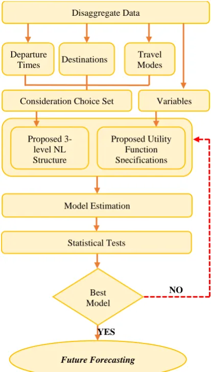
This research represents all of departure time (time of day), destination and travel mode choices under a unified model through using 3-level NL model in order to represent an effective and more accurate alternative approach for the first three steps in the 4-step travel demand model (generation, distribution and modal split). NL model is a disaggregate-based discrete choice model that relaxes the IIA property in MNL model by accounting for the correlation of error terms among similar alternatives [37]. To attain that, number of 3-level nesting structures that may describe the structure of the error distributions for alternative utilities has been developed. Figure 1 shows the general framework of the proposed model.
In order to test the significance of the proposed model, a simple MNL model that assumes identical cross-elasticity among all possible combinations is proposed to be estimated.
For MNL model, Equations (1) and (2) represent the general form of the total random utility function associated with alternatives.
Ui,tdm= Vi,tdm + Ԑi,tdm (1)
V i,tdm =ASCi,tdm+
α
*Qi,tdm+β*Ci (2)We assume an independent identical extreme value
distribution (Gumbel Type I) for the error terms Ԑtdm with
scale parameter θ and allocation parameter η=0 (For the sake of simplicity, the abbreviation “i” has been dropped from the rest of the text). Thus, joint probability can be expressed as shown in Equations (3) and (4).
P[tdm] =Pr [Vtdm - Vuen ≥ Ԑ uen - Ԑtdm], ∀ [u ϵ T, e ϵ D
and n ϵ M] (3)
where; Var(Ԑtdm)= 𝜋 2𝜃2
6 (4)
Therefor Equation (5) can represent the probability function of choosing travelling at departure time “t” to destination “d” using mode “m” from the choice set of T*D*M alternatives is:
P[tdm|TDM] = 1
1+∑T,D,Mu,e,nexp(Vuen|TDM− Vtdm|TDMθ ) ,
∀ [u ϵ T, e ϵ D and n ϵ M]
(5)
According to above equation, in MNL model, just difference between deterministic utility functions is matter and thus, it is possible to normalize scale parameter to the unity (Equation (6)).
P[tdm|TDM] = 1
1+∑T,D,Mu,e,n exp(Vuen|TDM− Vtdm|TDM) ,
∀ [u ϵ T, e ϵ D and n ϵ M]
(6)
In NL models, alternatives that are more similar in attributes and characteristics are grouped (or nested) with
Figure 1. General Framework of the proposed approach
Proposed Utility Function Specifications
Model Estimation
Best Model
Future Forecasting
Consideration Choice Set Departure
Times Destinations
Travel Modes
Variables Disaggregate Data
Statistical Tests
NO
YES
each other and formed exclusive subsets (nests). That means; alternatives in the same nest have a higher level of similarity and competitiveness than alternatives in different nests. Statistically, this can be achieved by imposing a random component (error term) to be common for all alternatives in the same nest and differs within nests. Such a random component ensures identical cross elasticity for all pairs of alternatives only in the same nest (subset) rather than being identical for all pairs of alternatives in the choice set like MNL model. Any potential correlation structures between groups of alternatives can be represented through developing associated nesting structures (tree structure).
Therefore, in order to properly represent the correlation between departure time, destination and travel mode, a set of proposed 3-level nesting structures have to be constructed. In which, each travel dimension can be settled at a specific level with Gumbel distribution for error terms that is IID within the same nest or the same sub-nest. For instance, departure time alternatives may be located at the highest level, destination alternatives may be placed at mid-level and travel mode at the lowest one. This structure can be interpreted by assuming that, individuals are firstly deciding on at which time to travel and therefore, they determine to which destination and finally they choose the travel mode. Moreover, on the context of correlation, this structure assumes similarity between alternatives belong to the same departure time nest. Intuitively, this assumption is accurate if time of day affects significantly and equally the unobserved attributes associated with destinations and modes such as safety and comfort. Moreover, inner correlation in the same travel dimension (e.g. similarities between public transportation modes in the travel mode) can be represented at a specific level, travel dimension itself at another and combinations of the other two travel dimensions placed at the third level.
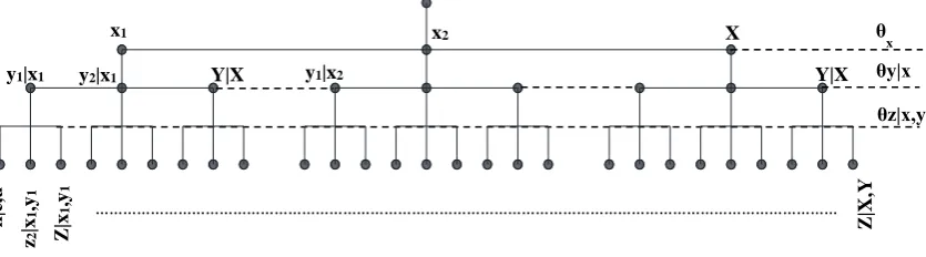
In order to express the probability functions associated with the proposed 3-level NL structures; we assume a 3-level nesting structure where different trip dimensions (x, y and z) can be located at different levels (Figure 2). Based on Figure 2, Equations (7) and (8) can represent the general forms of the utility functions associated with elementary alternatives;
Uz|x,y = Vz|x,y + Ԑx + Ԑ`y|x + Ԑ` z|y,x (7)
Vz|x,y =ASCz|x,y + α*Qz|x,y + β*Ci (8)
Equations (9), (10) and (11) show the variance of error terms at level 1, 2 and 3, respectively.
Var(Ԑ z|y,x)=
π2θ
z|y,t 2
6
Var(Ԑy|x)=
π2θ
y|x 2
6
(9)
(10)
Var(Ԑ x)=π 2θ
x 2
6 (11)
Consequently, the general forms of the joint probability of choosing x, y and z from a choice set of X*Y*Z alternatives can be expressed through Equations (12), (13) and (14).
𝑃[𝑥𝑦𝑧] = 𝑃[𝑥]𝑃[𝑦|𝑥]𝑃[𝑧|𝑦. 𝑥] = exp(
𝜃𝑦|𝑥 𝜃𝑥𝐼𝑦|𝑥)
∑ exp(𝜃𝑦|𝑥
𝜃𝑥𝐼𝑦|ℎ) 𝑋
ℎ
∗
exp(𝜃𝑧|𝑦.𝑥
𝜃𝑦|𝑥𝐼𝑧|𝑦.𝑥)
∑ exp(𝜃𝑧|𝑦.𝑥
𝜃𝑦|𝑥𝐼𝑧|𝑗.𝑥) 𝑌|𝑥
𝑗|𝑥
, ∗
exp(𝑉𝑧|𝑦.𝑥
𝜃𝑧|𝑦.𝑥)
∑ exp(𝑉𝑓|𝑦.𝑥
𝜃𝑧|𝑦.𝑥) 𝑍|𝑦.𝑥
𝑓|𝑦.𝑥
(12)
where, 𝐼𝑦|𝑥= ln ∑ exp (
𝜃𝑧|𝑦.𝑥
𝜃𝑦|𝑥𝐼𝑧|𝑗.𝑥)
𝑌|𝑥
𝑗|𝑥 , (13)
𝐼𝑧|𝑦.𝑥= ln ∑ exp (
𝑉𝑓|𝑦.𝑥
𝜃𝑧|𝑦.𝑥)
𝑍|𝑦.𝑥
𝑓|𝑦.𝑥 (14)
One of the most key features of the proposed approach over the traditional 4-step model is considering decision makers’ characteristics while modelling destination choice. Clearly, neglecting the socio-demographic characteristics of travellers can lead to insufficient models which cannot deal with the potential dynamics during the different planning horizons [38].
The variables Iy|x and Iz|y,x has a very important
interpretation. In literatures, it is referred to by various terms; Inclusive Value “IV”, Log-Sum, Expected Maximum Utility “EMU”, or Expected Consumer Surplus “ECS”. We consider the term inclusive value IV in the context. IV represents average utility which obtained by population in case of choosing any alternative within the specific nest. The existence of scale
parameter θz|y,x or θy|x in the denominator of IV equation
is the source of similarity between alternatives within a nest. By word, different scale parameters among nests lead to different IV’s which leads to different cross elasticity between those nests. Moreover, as scale parameter decreases IV increases and thus the sensitivity of choosing alternatives in that nest is more than choosing alternatives in other nests. That leads to a higher cross elasticity for alternatives with higher correlation.
Figure 2. A Proposed Nesting Structure for Connecting x, y and z by Three-Level NL Model
since the variance of mid-level should be more than or equal to the variance of lowest level, the scale parameters of the lowest level should be less than or equal to the scale parameter at mid-level. The opposite is right, where if the scale parameter of elementary alternatives is assumed to equal one, then the scale parameter of up-levels must be more than or equal to one. Moreover, under all conditions the values of scale parameter have to be non-negative to assure a concave single optima maximum likelihood function. In this research, we adopt the first setting through normalizing the scale parameter at top level to one. Therefore, the probability function takes the form of Equation (15).
𝑃[𝑥𝑦𝑧] = exp(𝜃𝑦|𝑥𝐼𝑦|𝑥)
∑ exp(𝜃𝑋ℎ 𝑦|𝑥𝐼𝑦|ℎ)
∗
exp(𝜃𝑧|𝑦.𝑥
𝜃𝑦|𝑥𝐼𝑧|𝑦.𝑥)
∑ exp(𝜃𝑧|𝑦.𝑥
𝜃𝑦|𝑥𝐼𝑧|𝑗.𝑥) 𝑌|𝑥
𝑗|𝑥
∗
exp(𝑉𝑧|𝑦.𝑥
𝜃𝑧|𝑦.𝑥)
∑ exp(𝑉𝑓|𝑦.𝑥
𝜃𝑧|𝑦.𝑥) 𝑍|𝑦.𝑥
𝑓|𝑦.𝑥
where, 0,00 ≤ 𝜃𝑧|𝑦.𝑥≤ 𝜃𝑦|𝑥≤ 1,00
(15)
4. CASE STUDY
In this paper, the proposed model will be estimated and calibrated by using shopping and entertainment trips data of Eskisehir city, Turkey. Notably, several studies have directed their attention toward examining different aspects of compulsory trips (work trips) rather than shopping and entertainment trips. Obviously, they were motivated by the demonstration of commuter trips on the daily congestion [39]. However, some other little literatures have directed their studies toward examining individuals’ behaviour while performing discretionary trips [40]. We adopt the second framework of studying shopping and entertainment trips as discretionary trips due to the following reasons;
• Discretionary trips establish a considerable proportion of the total daily trips with speculations predict a growing contribution to traffic congestion and mobile source emissions.
• Among evening peak-period trips, discretionary trips are found to occupy the first grad between all other trip purposes [41].
• Discretionary trips’ departure times and destinations are more likely to be shifted by individuals than work trips which have a more restricted time and space spans. In other words, compulsory trips (e.g. work trips) have less flexibility to make a change in departure time and destination.
The considered shopping and entertainment trips data are a part of large-scale revealed preference data which are collected through a household survey in 2015 in the context of Eskisehir master plan project which operated
by Eskisehir Metropolitan Municipality. From
approximately 10,000 households in the city, variety of data has been obtained. These data include;
(1) Household socio-demographics (household size, income, and vehicle ownership),
(2) Individual socio-demographics (gender, age, license holding to drive, and employment status),
(3) Individual’s travel information (departure time(s), purpose of the trip(s), origin(s) and destination(s)) (4) Attributes of used transportation mode(s) (out of vehicle travel time, in vehicle travel time and fare).
The total number of observations was around 30,000 of which about 12,000 observations are related to discretionary trips distributed among different departure times, destinations (about 190 destinations) and travel modes (10 modes; car, public bus, tramway, minibus, taxi, service, motorcycle, bicycle, walk and other). In this research, we focus our analysis on entertainment and shopping trips with specific number of times of day, destinations and transportation modes. By words, for those who travel to shopping and entertainment trip, time of day has been categorized into three different groups that differ among each other in terms of traffic conditions and availability of individual’s free times; peak time trips (p) [morning-peak 7.00am and 9.00am, and noon-peak 4.30pm and 6.30pm], off-Peak time trips (o) [9.00am and 4.30pm] and Evening time trips (e)[6.30pm up to 10.00pm]. Notably, observations outside these three
Z|
x1 ,y1
Z|
X,Y
k
|e
,u
x1 x2 X
y1|x1 y2|x1 Y|X
z
2
|x
1
,y
1
y1|x2 Y|X
θz|x,y θy|x θ
x
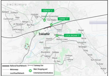
periods have been neglected since they are trivial and happen after mandatory closing hours of shopping and entertainment places (i.e. 10.00 pm). On the other hand, by considering only entertainment/shopping trips, the most attracted destinations are observed in three central areas which distinguished by having a lot of retail and entertainment activities. These destinations are; Espark shopping centre (s), Ozdilek shopping centre (z) and Local Bazaar (l) as illustrated in Figure 3. In the context of transportation mode, three modes that access to the three destinations and available during the three times of day have been considered in our analysis. These modes are private car (c), public bus (b) and tramway (tr). Eventually, by determining the choice set of each travel dimension available for each individual, the total number of observations has been found to be 529 observations. The distribution of individuals among available alternatives of each choice subset is shown in Table 1.
Regarding the preferences of time, surprisingly, more than half of observations (52.36%) were found preferring off-peak time period (9.00 am – 4.30 pm) to achieve their recreation trips. However, this result is consistent with the high portion of non-workers/ housewives in the sample which reaches 53.12% as illustrated in Table 2. On the other hand, about 28% of individuals prefer evening time to execute their shopping and entertainment activities. Obviously, they choose to go after normal work hours with enough amount of time to avoid congestion associated with commuter trips. Furthermore, individuals are less likely to choose peak periods to make their discretionary trips (only 19.66%). This result reflects the non-obligatory nature of discretionary trips without specific limitations in departure times which leads individuals to avoid high traffic volumes associated with peak periods.
Examining destination choices expresses that, in Eskisehir city, individuals who want to accomplish shopping or entertainment activities will most likely travel towards Bazaar region or Espark shopping centre (38.4 and 34.8% respectively) while Ozdilek shopping centre is less likely to be chosen (26.8%). Remarkably, while individuals travel to perform discretionary trips, distance between origin and destination is not the most significant factor that affects the distribution of trips among destinations. In our case, reviewing average distances between each trip origin and the chosen destination of each individual leads to the same result (Table 3). That is, despite Espark has the longest average travel distance from travel origins (5.10 Km), it attracts considerable share of trips like Local bazaar which has the lowest average travel distance (4.00 Km). At the same time, average travel distance from trip origins to Ozdilek is 4.10 Km which near to the distance to Bazaar, however, individuals are less likely traveling to it. Other factors such as travel time, travel cost, accessibility, density of shopping and entertainment activities are more crucial while deciding on destination of discretionary
trip. Of course, some of these factors could be examined through the proposed nested model. Notably, this is a core benefit for the proposed approach over the conventional 4-step model where actual individuals’ perceptions toward characteristics of alternatives are used rather than the average values. That results in more behavioural-based forecasting models which leads to more accurate future policy implications.
Figure 3. Map of the Study Area
TABLE 1. Sample Distributions among Alternatives
# of Observations Rate %
Departure time (t)
Peak (p) 104 19.66
Off-Peak (o) 277 52.36
Evening (e) 148 27.98
Destination (d)
Espark (s) 184 34.78
Local Bazaar (l) 203 38.37
Ozdilek (z) 142 26.84
Travel modes (m)
Car (c) 116 21.93
Bus (b) 98 18.53
Tramway (tr) 315 59.55
TABLE 2. Distribution of Sample According to Work Status
# of Observations Rate %
Doesn’t work or housewife 281 53.12
Works or a student 248 46.88
TABLE 3. Average Travel Distance to the Destinations
Row Labels Average Distance (Km)
Espark (s) 5.1
Local bazaar (l) 4.0
Finally, the modal split of shopping and entertainment trips is 21.9, 18.5 and 59.6% for car (c), bus (b) and tramway (tr), respectively. More than half of individuals do prefer tramway over other modes while
traveling to discretionary trips. However, this
distribution is totally different when comparing with modal split of work trips which is 63, 15 and 22% for car, bus and tramway respectively. Obviously, individuals’ behaviour while choosing among travel modes is strongly correlated with trip purpose since other factors may be included while decide traveling to shopping places such as availability of parking places, parking fees, activity time, flexibility of both departure and arriving times, etc. Such factors and more can be examined and investigated by representing it through the utility functions of alternatives.
5. MODELS ESTIMATION
The total number of alternatives equals 27 (the possible combinations of 3 times [p, o, e], 3 destinations [s, l, z] and 3 transportation modes [c, b, tr]). Additionally, linear in parameters utility functions have been assumed which consider total travel time TT and total travel cost TC as alternative’s attributes and monthly income group INC, age AGE, car ownership COW (dummy variable) and student status SS (dummy variable) as socio-demographic characteristics of individuals.
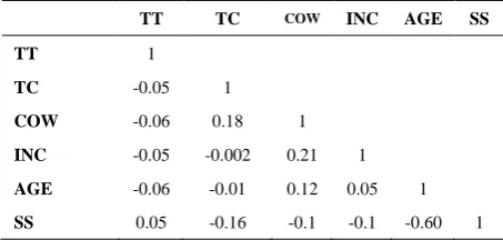
Furthermore, in order to check the multi-collinearity, the correlation among all variables has been calculated (Pearson correlation coefficients). Table 4 shows the correlation matrix of the variables. As illustrated, the correlation between all pairs of the variables is low (weak) except for age-student status where correlation has a moderate (intermediate) value [42]. Therefore, all proposed variables can be used efficiently to estimate the proposed models.
Moreover, for all proposed nesting structures, in the light of descriptive statistics, different specifications for the available variables have been introduced in order to capture the best model for each structure in terms of the magnitude of inclusive value parameters, signs and degree of significance of parameters as well as the overall
TABLE 4. Correlation Matrix of the Proposed Variables
TT TC COW INC AGE SS
TT 1
TC -0.05 1
COW -0.06 0.18 1
INC -0.05 -0.002 0.21 1
AGE -0.06 -0.01 0.12 0.05 1
SS 0.05 -0.16 -0.1 -0.1 -0.60 1
goodness of fit of the model. That is, for each proposed structure, different combinations of generic and alternative specific variables have been assumed. Notably, representing alternative specific parameters means a total number of parameters equal to the total number of alternatives (total number of alternatives minus one, in our example equals 26). Introducing this large number of estimates will not only add more encumbrances in estimation process but also complicate the interpretation of the results. Therefore, in an attempt to intuitively interpret results of estimation as well as ease the estimation process, the alternative specific variables (especially those related to individual characteristics) have been represented to be particular to a specific travel dimension(s) rather than the all 27 alternatives. For instance, in some specifications, the parameter of age variable has been presumed to be specific to time of day alternatives. However, in other specifications, it has been assumed to be specific to destination or transportation mode alternatives and therefore, best specifications that lead to best models are selected.
6. DISCUSSION OF ESTIMATION RESULTS
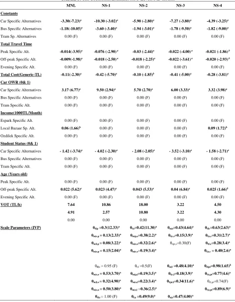
In order to properly represent the correlation between time of day, destination and transportation mode, a set of the proposed 3-level nesting structures is estimated. In which, each travel dimensions could be settled at a specific level with Gumbel distribution for error terms that are IID within the same nest or the same sub-nest. Moreover, inner correlation in the same travel dimension (e.g. similarities between bus and tramway in the transportation model travel dimension) can be represented at a specific level. For all proposed nesting structures, the scale parameters at upper level have been normalized to 1.00. In the light of the estimation process, 4 proposed 3-level NL structures have been found representing acceptable estimates with remarkable goodness of fit. The best 4 models are appointed as NS-1, NS-2, NS-3 and NS-4. Notably, these models are associated with the same utility function specifications which are illustrated in equation 16. Furthermore, Table 5 shows the estimation results of the four proposed NL structures.
Vt,d,m=ASCm+𝑏𝑇𝑇𝑡 *TT+𝑏𝑇𝐶*TC+𝑏𝐶𝑂𝑊𝑚 *COW+𝑏𝐼𝑁𝐶𝑑 *INC+𝑏𝑆𝑆𝑚*SS+𝑏𝐴𝐺𝐸𝑡 *AGE
(16)
tramway alternatives at specific levels where; NS-3 considers destinations at top, transportation modes with two specific branches at mid-level (private car and public transportations) and departure times at the lower level. NS-4, however, treats transportation modes at upper level
with two branches (private car and public
transportations), destinations and departure times follow at mid and lower levels, respectively.
According to estimation results, the following conclusions can be figured out:
• In terms of overall goodness of fit, the 4 proposed models achieve acceptable values where log likelihood
ratios exceed the critical χ2 at 5% level of significance
• Regarding scale parameters, in the 4 models, all values are in between the acceptable ranges where; by normalizing scale parameters at top levels, the mid-level
scale parameters (e.g. θd|p, θd|o and θd|e in NS-1) are less
than or equal to one and more than zero. However, the
lower level scale parameters (e.g. θm|s,p, θm|l,p and θm|z,p
in NS-1) are less than or equal to the parameters of the mid-level and more than zero (e.g. 1.00 > θd|t > θm|d,t
>0.00).
• The signs of departure time specific estimates of travel time are consistent for all models (negative). The magnitudes, however, are more coherent in NS-1 and NS-2 than NS-3 and NS-4. In NS-1 and NS-2, the magnitudes of travel time estimates reflect that while performing shopping and entertainment trips, individuals of Eskisehir perceive more importance for total travel time in peak periods than off-peak periods, nevertheless, NS-3 and NS-4 suggest equal perceptions for both times. • The negative signs of the generic total cost parameters in all models indicate intuitively the inclination of decreasing utilities of shopping and entertainment trips as travel cost increases.
• The mode specific estimates of car ownership associated with private car have positive sings (as expected) in all of 4 models which lead to the fact that the availability of private car increases the likelihood of using private car over public transportation to shopping and entertainment destinations.
• The income parameters (specific to destination) turn to be insignificant in all models except for NS-4 where the Local Bazaar specific income parameter is significant at 10%, however, the positive sign related to it leads to illogic interpretation where it suggests that individuals with higher monthly income are more likely prefer doing shopping in Local Bazaar than shopping malls.
• Specific to private car mode, being a student represents a significant variable with negative parameter for all models. Obviously, while applying shopping and entertainment trips, being a student increase the probability of using public transportation modes over private car.
• The estimates of Age variable are significantly different than zero and have positive signs in all models. Specific to departure time, getting older decreases the probability
of performing shopping and entertainment trips at peak periods and evening as well.
• Reviewing the value of time “VOT” leads to conclude that, models of NS-1 and NS-2 have more reliable values than models of NS-3 and NS-4 where individuals generally perceive more willingness to pay at peak periods over at off-peak periods rather than similar perceptions at both periods. Furthermore, the magnitudes of VOT in NS-1 (10.86 TL/h at peak, 2.57 at off-peak and 0 at evening) may be more reasonable than their magnitudes in NS-2 (18.00 TL/h at peak, 10.80 at off-peak and 0 at evening) where the magnitude of VOT at peak in the former is closer to average hourly wage rate which equals about 12 TL/h (average monthly income is 2160 TL, 22 work days and 8 hours working per day). • The 4 proposed 3-level NL models are developed significantly over the less advanced MNL where the values of log likelihood ratio of 3-level relative to the
MNL exceed the critical χ2 at 5% level of significance
and different degree of freedoms.
• Maximum of maximum log likelihood value is associated with NS-1 (-1512.57) with highest log likelihood ratio relative to the MNL model (54.90). That may lead to conclude that for shopping and entertainment trips, individuals in Eskisehir city are more likely deciding at first on departure time which follows by deciding on destination which follows by transportation modes.
• From another hand, the value of maximum log likelihood of model NS-2 (-1521.78) is slightly lesser than the maximum one of NS-1 with acceptable signs and magnitudes for estimates and VOT. That sheds the light on a considerable portion of sample that may consider the proposed nesting structure NS-2 as a decision role while travelling to shopping and entertainment trips (destination, then time of day, then transportation mode). The existence of two different nesting structures with close overall goodness of fit can be interpreted as a portion of heterogeneity in the sample (as presenter to the overall population) which can be considered with more advanced choice models; however, this approach is out of the scope of this research.
• The models NS-3 and NS-4 are arguable to be accepted even if they have a considerable LL value with significant LL ratio relatively to the less advanced MNL model. The main reason is the equal values associated with the departure time specific travel time estimates which lead to equal VOTs for both peak and off-peak periods as illustrated previously. Moreover, the positive sign of income variable parameter for Local Bazaar in NS-4 is against intuition.
TABLE 5. The Coefficient Estimates for 3-Levels NL models
MNL NS-1 NS-2 NS-3 NS-4
Constants
Car Specific Alternatives -3.30(-7.23)a -10.30 (-3.02)a -5.90 (-2.80)a -7.27 (-3.80)a -4.39 (-3.25)a
Bus Specific Alternatives -1.18(-10.05)a -3.60 (-3.40)a -1.94 (-3.01)a -1.78 (-9.50)a -1.82 (-9.00)a
Tram Sp. Alternatives 0.00 (F) 0.00 (F) 0.00 (F) 0.00 (F) 0.00 (F)
Total Travel Time
Peak Specific Alt. -0.014(-3.95)a -0.076 (-2.90) a -0.03 (-2.44)a -0.022 (-4.00) a -0.021 (-1.86) b
Off-peak Specific Alt. -0.009(-1.98)a -0.018 (-2.50) a -0.018 (-2.25)a -0.022 (-3.61) a -0.020 (-2.93) b
Evening Specific Alt. 0.00 (F) 0.00 (F) 0.00 (F) 0.00 (F) 0.00 (F)
Total Cost(Generic-TL) -0.11(-2.30)a -0.42 (-5.70)a -0.10 (-1.85)b -0.41 (-5.00)a -0.28 (-3.81)a
Car OWR (0& 1)
Car Specific Alternatives 3.17 (6.77)a 9.50 (2.94)a 5.70 (2.70)a 6.00 (3.33)a 3.32 (3.98)a
Bus Specific Alternatives 0.00 (F) 0.00 (F) 0.00 (F) 0.00 (F) 0.00 (F)
Tram Specific Alt. 0.00 (F) 0.00 (F) 0.00 (F) 0.00 (F) 0.00 (F)
Income(1000TL/Month)
Espark Specific Alt. 0.00 (F) 0.00 (F) 0.00 (F) 0.00 (F) 0.00 (F)
Local Bazaar Sp. Alt. 0.06 (1.66)b 0.00 (F) 0.00 (F) 0.00 (F) 0.09 (1.72)b
Ozdilek Specific Alt. 0.00 (F) 0.00 (F) 0.00 (F) 0.00 (F) 0.00 (F)
Student Status (0& 1)
Car Specific Alternatives - 1.42 (-3.74)a - 4.02 (-2.30)a - 2.08 (-2.05)a - 3.52 (-3.10)a - 1.58 (-2.71)a
Bus Specific Alternatives 0.00 (F) 0.00 (F) 0.00 (F) 0.00 (F) 0.00 (F)
Tram Specific Alt. 0.00 (F) 0.00 (F) 0.00 (F) 0.00 (F) 0.00 (F)
Age (Years old)
Peak Specific Alt. 0.00 (F) 0.00 (F) 0.00 (F) 0.00 (F) 0.00 (F)
Off-peak Specific Alt. 0.022 (5.62)a 0.023 (4.47)a 0.043 (5.53)a 0.04 (6.84)a 0.025 (1.66)b
Evening Specific Alt. 0.00 (F) 0.00 (F) 0.00 (F) 0.00 (F) 0.00 (F)
VOT (TL/h) 7.64 10.86 18.00 3.22 4.50
4.91 2.57 10.80 3.22 4.30
0.00 0.00 0.00 0.00 0.00
Scale Parameters (IVP) θd|p =0.3(12.33)a θt|s=0.42(11.30)a θm|s=0.43(4.64)a θd|c=0.63(2.63)a
θm|s,p = 0.13(2.33)a θm|p,s=0.38(2.2)a θt|c,s=0.15(3.9)a θt|s,c=0.31(2.7)a
θm|l,p = 0.08(3.22)a θm|o,s=0.32(2.6)a θt|pt,s=0.30(F) θt|l,c=0.28(3.4)a
θm|z,p = 0.15(2.04)a θm|e,s=0.19(3.4)a θt|z,c = 0.40(2.6)a
θd|o = 0.95 (F) θt|l =0.5(F) θm|l =0.48(4.10)a θd|pt=0.98(1.65)b
θm|s,o = 0.53(3.70)a θm|p,l=0.19(3.5)a θt|c,l=0.18(3.9)a θt|s,pt=0.77(4.6)a
θm|l,o = 0.32(4.90)a θm|o,l=0.22(3.4)a θt|pt,l=0.34(11.6)a θt|l,pt=0.74(F)
θm|z,o = 0.50(3.80)a θm|e,l =0.36(2.5)a θt|z,pt=0.89(6.9)a
θm|s,e = 0.30(3.30)a θm|p,z=0.43(1.65)b θt|c,z=0.15(4.3)a
θm|l,e = 0.25(3.80)a θm|o,z=0.27(2.9)a θt|pt,z=0.43(8.8)a
θm|z,e = 0.29(3.40)a θm|e,z =0.29(2.7)a
# of Observations 529 529 529 529 529
# of estimates 9 19 20 17 16
LL(0) NA -1743.50 -1743.50 -1815.30 -1815.30
LL(β) -1540.02 -1512.57 -1521.04 -1517.78 -1532.54
LL(C) -1666.90 -1655.13 -1655.53 -1655.90 -1621.87
-2LL[βvs.C] (χ2=14.1) 253.76 285.12 268.98 276.24 178.66
ρ2(βvs.C) 0.076 0.086 0.081 0.083 0.055
-2LL [vs.MNL] NA 54.90 37.96 44.48 14.96
χ2(df) - 18.31 (df=10) 19.68 (df=11) 15.51 (df=8) 14.10 (df=7)
F=Fixed Parameter, NA= Not Applicable, a Significant at 95% level, b Significant at 90% level, t-statistics in parentheses
7. CONCLUSIONS
This research aims to represent departure time, destination and travel mode choices under a unified disaggregate model that can consider for the potential inter-correlation among them. In order to attain that,
1. Sumi, L. and Ranga, V., "Intelligent traffic management system for prioritizing emergency vehicles in a smart city", International
Journal of Engineering- Transaction A: Basics, Vol. 31, No. 2,
(2018), 278-283.
2. Ghasemi, J. and Rasekhi, J., "Traffic signal prediction using elman neural network and particle swarm optimization", 8. REFERENCES
Finally, our proposed model has succeeded in representing disaggregate behaviour for limited number of travel dimensions (e.g. 3 times, 3 destinations and 3 modes) which makes it reliable and more accurate for small-scale planning issues. However, it has the capability to analyse large-scale planning horizons by calibrating it with aggregate-data.
connectivity among different travel choices that are common in the same trip (e.g. time of day, destination and transportation mode) rather than treating them separately as 4-step model does. Obviously, in the light of the estimation results, the relative values of scale parameters support that decision makers are more likely decide on different travel choices jointly rather than separately. Therefore, neglecting such dependency (correlation) may lead to insufficient and inconsistent models. That can be clearly demonstrated through comparing the results of the proposed model with other studies which did not consider correlation between different travel dimensions. For example, the model proposed by Bowman and Ben-Akiva [30] has connected departure times from one side with the combinations of destinations and travel modes from the other without accounting for associated correlations. The estimation results of the model’s prototype that was introduced for Boston are found to have some faults. For instance, unrealistic estimates for VOT have obtained.
Overall, the 3-level NL model achieves the discrete 3-level NL model is suggested to be used.
Through it, different potential correlation patterns were constructed via the associated nesting structures. The proposed model provided a reliable and applicable alternative representation that can substitute the first 3-steps in the traditional 4-step model. The formulated models have been examined on disaggregate shopping and entertainment travels’ data that are obtained in 2015 from Eskisehir city’s household survey, Turkey.
The estimation results lead to significant conclusions which may be summarized in the following points: • Opposite to 4-step model, the proposed model shows adequate flexibility in accounting for attributes of alternatives and characteristics of decision makers as well which results in a more consistent behavioural travel demand representation.
• Moreover, our proposed approach provides behavioural-based simulation instrument that can be used to test various hypothetical situations to precisely predict future travel demand preferences under temporal, spatial, socio-economic and demographic changes.
International Journal of Engineering-Transactions B:
Applications, Vol. 29, No. 11, (2016), 1558-1564.
3. Johnston, R., "The urban transportation planning process", The
Geography of Urban Transportation, Vol. 3, (2004), 115-140.
4. Morehouse, T.A., "The 1962 highway act: A study in artful interpretation", Journal of the American Institute of Planners, Vol. 35, No. 3, (1969), 160-168.
5. Boyce, D., "Is the sequential travel forecasting paradigm counterproductive?", Journal of Urban Planning and
Development, Vol. 128, No. 4, (2002), 169-183.
6. Gu, Y., "Integrating a regional planning model (transims) with an operational model (corsim)", Virginia Tech, (2004),
7. Bhat, C.R., "Analysis of travel mode and departure time choice for urban shopping trips", Transportation Research Part B:
Methodological, Vol. 32, No. 6, (1998), 361-371.
8. Stopher, P.R., "Deficiencies of travel-forecasting methods relative to mobile emissions", Journal of Transportation
Engineering, Vol. 119, No. 5, (1993), 723-741.
9. Weiner, E., "Upgrading travel demand forecasting capabilities", in 4th National Conference on Transportation Planning Methods Applications, Volumes I and II. A Compendium of PapersTransportation Research Board Committee on Transportation Planning Applications-A1C07; Federal Highway Administration; Federal Transit Administration; McTrans Center, University of Florida; and hosted by the Florida Department of Transportation., (1993).
10. Setak, M., Dastaki, M.S. and Karimi, H., "Investigating zone pricing in a location-routing problem using a variable neighborhood search algorithm", International Journal of
Engineering-Transactions B: Applications, Vol. 28, No. 11,
(2015), 1624-1633.
11. Ben-Akiva, M.E., Lerman, S.R. and Lerman, S.R., "Discrete choice analysis: Theory and application to travel demand, MIT press, Vol. 9, (1985).
12. McNally, M.G., "The four step model", In: Handbook of Transport Modelling, ed. David A. Hensher and Kenneth J. Button, (2000), 35-52.
13. Oppenheim, N., "Urban travel demand modeling: From individual choices to general equilibrium, John Wiley and Sons, (1995).
14. Vuchic, V.R., "Urban transit: Operations, planning, and economics, John Wiley & Sons, (2017).
15. Donnelly, R., "Advanced practices in travel forecasting, Transportation Research Board, Vol. 406, (2010).
16. Small, K.A., "The scheduling of consumer activities: Work trips",
The American Economic Review, Vol. 72, No. 3, (1982),
467-479.
17. Hendrickson, C. and Plank, E., "The flexibility of departure times for work trips", Transportation Research Part A: General, Vol. 18, No. 1, (1984), 25-36.
18. Wilson, P.W., "Scheduling costs and the value of travel time",
Urban Studies, Vol. 26, No. 3, (1989), 356-366.
19. Noland, R. and Small, K.A., "Travel-time uncertainty, departure time choice, and the cost of morning commutes", Transportation
Research Record, Vol. 1493, (1995), 150-158.
20. Abu-Eisheh, S. and Mannering, F.L., "Discrete/continuous analysis of commuters' route and departure time choices",
Transportation Research Record, Vol. 1138, (1987), 27-34.
21. Hamed, M.M. and Mannering, F.L., "Modeling travelers' postwork activity involvement: Toward a new methodology",
Transportation Science, Vol. 27, No. 4, (1993), 381-394.
22. Bhat, C.R. and Steed, J.L., "A continuous-time model of departure time choice for urban shopping trips", Transportation
Research Part B: Methodological, Vol. 36, No. 3, (2002),
207-224.
23. Wang, J.J., "Timing utility of daily activities and its impact on travel", Transportation Research Part A: Policy and Practice, Vol. 30, No. 3, (1996), 189-206.
24. Yamamoto, T., Fujii, S., Kitamura, R. and Yoshida, H., "Analysis of time allocation, departure time, and route choice behavior under congestion pricing", Transportation Research Record, Vol. 1725, No. 1, (2000), 95-101.
25. Ettema, D. and Timmermans, H., "Modeling departure time choice in the context of activity scheduling behavior",
Transportation Research Record, Vol. 1831, No. 1, (2003),
39-46.
26. Bhat, C.R., "A hazard-based duration model of shopping activity with nonparametric baseline specification and nonparametric control for unobserved heterogeneity", Transportation Research
Part B: Methodological, Vol. 30, No. 3, (1996), 189-207.
27. Bhat, C.R., "A multiple discrete–continuous extreme value model: Formulation and application to discretionary time-use decisions", Transportation Research Part B: Methodological, Vol. 39, No. 8, (2005), 679-707.
28. Bhat, C.R., "The multiple discrete-continuous extreme value (mdcev) model: Role of utility function parameters, identification considerations, and model extensions", Transportation Research
Part B: Methodological, Vol. 42, No. 3, (2008), 274-303.
29. Pinjari, A.R. and Bhat, C., "A multiple discrete–continuous nested extreme value (MDCNEV) model: Formulation and application to non-worker activity time-use and timing behavior on weekdays", Transportation Research Part B:
Methodological, Vol. 44, No. 4, (2010), 562-583.
30. Bowman, J.L. and Ben-Akiva, M.E., "Activity-based disaggregate travel demand model system with activity schedules", Transportation Research Part A: Policy and
Practice, Vol. 35, No. 1, (2001), 1-28.
31. You, D., Garikapati, V.M., Konduri, K.C., Pendyala, R.M., Vovsha, P. and Livshits, V., Multiple discrete-continuous model of activity type choice and time allocation for home-based nonwork tours. (2013).
32. Bhat, C.R., "Accommodating flexible substitution patterns in multi-dimensional choice modeling: Formulation and application to travel mode and departure time choice", Transportation
Research Part B: Methodological, Vol. 32, No. 7, (1998),
455-466.
33. McFadden, D., "Modeling the choice of residential location",
Transportation Research Record, Vol. 673, (1978).
34. Jrew, B., Msallam, M. and Momani, M., "Strategic development of transportation demand management in jordan", Civil
Engineering Journal, Vol. 5, No. 1, (2019), 48-60.
35. Moradzaeh, A. and Khaffafi, K., "Comparison and evaluation of the performance of various types of neural networks for planning issues related to optimal management of charging and discharging electric cars in intelligent power grids", Emerging Science
Journal, Vol. 1, No. 4, (2018), 201-207.
36. Shafiei, S., Vaelizadeh, R., Bertrand, F. and Ansari, M., "Evaluating and ranking of travel mode in metropolitan; a transportation economic approach", Civil Engineering Journal, Vol. 4, No. 6, (2018), 1303-1314.
37. Koppelman, F. and Bhat, C., "A self instructing course in mode choice modeling: Multinomial and nested logit models. Prepared for us department of transportation federal transit administration",
38. McNally, M.G., "The potential for integrating gis in activity-based forecasting models", Center for Activity Systems Analysis, University of California. (1997).
39. Mahmassani, H.S. and Jou, R.-C., Bounded rationality in commuter decision dynamics: Incorporating trip chaining in departure time and route switching decisions, in Theoretical foundations of travel choice modeling. 1998, Pergamon.201-229.
40. Steed, J.L. and Bhat, C.R., Modeling departure time choice for home-based non-work trips. 2000, Southwest Region University Transportation Center, Center for Transportation.
41. Gordon, P., Kumar, A. and Richardson, H.W., "Beyond the journey to work", Transportation Research Part A: General, Vol. 22, No. 6, (1988), 419-426.
42. Salkind, N.J. and Frey, B.B., "Statistics for people who (think they) hate statistics, Sage Publications, Incorporated, (2019).
Application of Discrete 3-level Nested Logit Model in Travel Demand Forecasting
as an Alternative to Traditional 4-Step Model
M. Elmorssy, H. O. Tezcan
Istanbul Technical University, Faculty of Civil Engineering, Department of Transportation, Istanbul, Turkey
P A P E R I N F O
Paper history: Received 20 July 2019
Received in revised form 07 September 2019 Accepted 12 September 2019
Keywords:
Discrete Choice Models Departure Time Travel Demand Modelling Traditional 4-step Model Transportation Modes
هديكچ
رفس تلاح باختنا و دصقم ، تمیزع نامز هک دهد یم هئارا دیدج یزاس لدم دركیور کی یفرعم فده اب هلاقم نیا
یتنس لدم یاهدوبمک رب ناوت یم نآ قیرط زا .دهد یم ناشن هچراپكی بوچراچ کی تحت ار 4
مدع اب هارمه یا هلحرم
وت یم ار فده نیا .درک هبلغ نارفاسم یعقاو یاهراتفر یفرعم لدم ذاختا اب نا
3 هتسسگ
Logit Nested Logit
هک
لدم .تسا رفس تلاح یاه هنیزگ و دصقم ، تمیزع نامز نيب رد )عطاقتم ششک( فلتخم هوقلاب یگتسبمه رگنايب
رهش زا یرايتخا یاهرفس یاه هداد زا هدافتسا اب یداهنشيپ
Eskisehir
هب هجوت اب .تسا هدش شیامزآ و دروآرب هيکرت ،
جیاتن روط هب ات دنريگب ميمصت یرايتخا رفس داعبا دروم رد دنريگب ميمصت کرتشم روط هب دنراد لیامت دارفا ، نيمخت
یتنس لدم طسوت هک هناگادج 4
رد ار یرتشيب یریذپ فاطعنا یداهنشيپ دركیور ، نیا رب هولاع .دوش ضرف یا هلحرم
یاه یگژیو هارمه هب اه نیزگیاج یاه یگژیو نتفرگ رظن رد لدم کی هب رجنم نیا .دهد یم ناشن ناگدنريگ ميمصت
لدم .دوش یم رتشيب نانيمطا اب یتسايس یاهدمايپ و هدنیآ رت قيقد ینيب شيپ ، رت یراتفر یراتفر رفس یاضاقت یزاس
یارب یرت نئمطم و رت قيقد نیزگیاج یداهنشيپ 3
لدم لوا هلحرم 4
رد یزیر همانرب تاعوضوم رد یتنس یا هلحرم
ايقم ، رادیاپ یراتفر لدم کی هب یبايتسد تهج رد مهم فطع هطقن کی یداهنشيپ دركیور ، ماجنارس .تسا کچوک س
.تسا هدش ليكشت رفس یاضاقت داعبا همه زا هک تسا لماک سايقم رد هچراپكی و دمآراک