Please cite this article in press as:ParisaNiloofar, ParastooNiloofar, Yaseri M. Assessing diagnostic accuracy of doctors without a gold standard using Bayesian networks and K-modes clustering algorithm. J BiostatEpidemiol. 2019; 4(4): 184-195
J Biostat Epidemiol. 2019;4(4): 184-195
Original Article
Assessing diagnostic accuracy of doctors without a gold standard using Bayesian networks and
K-modes clustering algorithm
Parisa Niloofar1, Parastoo Niloofar2, Mehdi Yaseri2
1Department of Statistics, University of Bojnord, Bojnord, Iran.
2School of Public Health, Department of Epidemiology and Biostatistics, Tehran University of Medical Sciences, Tehran, Iran.
ARTICLE INFO ABSTRACT
Received 25.09.2018 Revised 19.10.2018 Accepted 23.01.2019 Published 14.03.2019
Key words:
Bayesian networks; Cluster Analysis; Diabetic Retinopathy; Humans; Sensitivity
Background & Aim: The diagnostic accuracy of a test is the ability to discriminate accuratelybetween patients who have and do not have the target disease. A common problem in assessing thediagnostic accuracy of doctors is the unknown true disease status which in the literature is referredas “absence of a gold standard”.
Methods & Material: In this article, a Naïve Bayesian network with hidden class node and a clusteringbased algorithm for categorical data named K-modes are proposed for estimating the diagnosticaccuracy of 5 physicians in diagnosing Diabetic Retinopathy. Also to assess and compare the efficiencies of these models, a simulation study with two different scenarios is conducted.
Results: Simulation study indicates that for Naïve Bayesian network and the non-rare disease, say forprevalence 0.1 and 0.2, as the sample size increases so the coverage probability. But for high prevalencevalues, say 0.5, coverage probabilities are not as good as those of non-rare disease. K-modes algorithm's efficiency decreases by the increase in the number of records, but it achieves betterresults when there are a small number of records, prevalence is approximately 0.3 and sensitivitiesare high. Results of the real data set reveal that sensitivities for all physicians except one, were higher than 85% and all specificities were higher than 90%. Also the estimated prevalence happensto be 0.32.
Conclusion: Through simulations and data analysis we show that this new approach based on Naïve Bayesian networks provides a useful alternative to traditional latent class modeling approaches usedin this setting.
.
Introduction
Diagnosis of a disease can sometimes be made on the basis of clinical signs and symptoms, but accurate diagnosis often requires the use of diagnostic tests. The evaluation of the accuracy of diagnostic testsis highly crucial and must be done on a relatively large sample of clinically suspected patients. Thediagnostic accuracy of a test is the ability to discriminate accurately between patients who have and do not have the target disease. Sensitivity and specificity are the most commonly used diagnostic testmeasures. Sensitivity is the proportion of diseased subjects
Corresponding author: Email: [email protected], Postal Address:
Department of Statistics, University of Bojnord, 4thkilometer road to
Esfarayen, Bojnord, North Khorasan province, Iran.
that show a positive test result. Specificityis the proportion of non-diseased subjects that show a negative test result. However, estimating thesediagnostic accuracy measures require information from the true disease status of the individuals which is determined by “gold standard” (1, 2). “Gold standard” test, is a test which is error free and perfectly classifies the patients into groups of diseased and non-diseased (3).
185 categoricaldata. In fact, cluster analysis is the
partitioning of similar objects into meaningful classes, when both the number of classes and the composition of the classes are to be determined (4, 5).
Cluster analysis is sometimes called latent class analysis (LCA) when the variables are categorical(6, 7). The k-modes clustering algorithm (8, 9) is one of the first algorithms for clustering large categorical data. In the past decade, this algorithm has been well studied and widely used in various applications.
When the gold standard is binary (disease and nondisease), methods have been proposed to estimate the accuracy of multiple binary tests without a gold standard (10). But to the best of our knowledge, no study has been done on applying Bayesian networks for diagnostic accuracy measurements. K-Modesclustering algorithm, have also received no attention in the context of diagnostic accuracy, and we show that it performs very weak comparing to Bayesian networks.
This paper is concerned with a special type of LC models called Naïve Bayesian networks with thebinary class node being hidden. Class node is the parent node of all other nodes and no other connectionsare allowed in a Naïve Bayesian network. This leads to the local independence
assumption, i.e., given the class variable, observed variables are independent of each other. In this paper, we propose a method to estimate the diagnostic accuracy of doctors without a gold standard using Naïve Bayesian networksfor which the true disease status is considered to be a binary latent variable. The proposed method is illustrated on a real data set from a study of Diabetic Retinopathy diagnosis data as well as a simulationstudy.
Method
We limit the discussion to the situation that a binary diagnostic test is used to diagnose a binary diseasestatus. Let yij be the observed binary
outcome (0= negative,1= positive) for the jth
imperfect test(or diagnoses from jth doctor) T j on
the ith subject with the unobservable true disease
status Di(0=not diseased, 1= diseased), where i =
1, 2,…,N, j = 1, 2,…, J, and yij is a realization of
the binary random variable Yij. The outcome
pattern over all tests for an individual subject i is then a vector yi of length J with yi= (yi1, yi2,
…,yiJ)T. Results for an individual test are
Bernoulli distributed with P(Yij= 1|Di= d), the
probability of testing positive on the jth test given
an individual's true diseasestatus d. The conditional independence assumption can be expressed as:
𝑃(𝑌𝑖1 = 𝑦1. 𝑌𝑖2 = 𝑦2. … . 𝑌𝑖𝐽 = 𝑦𝐽|𝐷𝑖 = 𝑑) = ∏ 𝑃(𝑌𝑖𝑗 = 𝑦𝑗|𝐷𝑖 = 𝑑) 𝐽
𝑗=1
(1)
This can be expressed in terms of the test sensitivities and specificities as:
𝑃(𝑌𝑖1 = 𝑦1. 𝑌𝑖2 = 𝑦2. … . 𝑌𝑖𝐽 = 𝑦𝐽|𝐷𝑖 = 1) = ∏ 𝑆𝑗𝑦𝑗 𝐽
𝑗=1
(1 − 𝑆𝑗)(1−𝑦𝑗) (2)
𝑃(𝑌𝑖1 = 𝑦1. 𝑌𝑖2 = 𝑦2. … . 𝑌𝑖𝐽 = 𝑦𝐽|𝐷𝑖 = 0) = ∏ 𝐶𝑗 (1−𝑦𝑗)
𝐽
𝑗=1
(1 − 𝐶𝑗)𝑦𝑗 (3)
with Sj= P(Yij= 1|Di= 1) = P(Yj= 1|Di= 1) being the sensitivity of test Tj and Cj=
186 The marginal distribution of Yi can be written as follows:
𝑃(𝒀𝑖) = ∑ 𝑃(𝑌1= 𝑦1. 𝑌2 = 𝑦2. … . 𝑌𝐽= 𝑦𝐽|𝐷𝑖= 𝑑) 1
𝑑=0
𝑃(𝐷𝑖= 𝑑)
= ∑ 𝑃(𝐷𝑖= 𝑑)
1
𝑑=0
∏ 𝑃(𝑌𝑗 = 𝑦𝑗|𝐷𝑖 = 𝑑) 𝐽
𝑗=1
= 𝜋 ∏ 𝑆𝑗𝑦𝑗
𝐽
𝑗=1
(1 − 𝑆𝑗)(1−𝑦𝑗)+ (1 − 𝜋) ∏ 𝐶
𝑗 (1−𝑦𝑗)
𝐽
𝑗=1
(1 − 𝐶𝑗)𝑦𝑗
(4)
where 𝜋 = 𝑃(𝐷𝑖 = 1) is the prevalence of the
disease. As you can see the test sensitivities and specificities remain constant (fixed effects model) from subject to subject. When the test sensitivities and specificities vary among the subjects it is called random effects model. The reason to perform the diagnostic study is to estimate the disease prevalence and the sensitivity and specificity of the tests.
Naïve Bayesian networks
When the true disease status is binary, sensitivity, specificity, positive and negative
predictive values are the parameters which describe the accuracy of different diagnostic tests or doctors. One of the simplest, and yet most consistently well-performing set of models that can be used for estimating these parameters is Naïve Bayesian network.
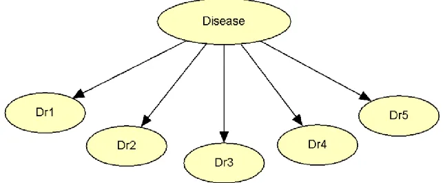
A Naïve Bayes, as discussed in (11), is a simple structure that has the classification node as the parentnode of all other nodes, see Figure (1). No other connections are allowed in a Naïve Bayes structure.
In this network the joint probability distribution of the variables is
𝑃(𝐷𝑖𝑠𝑒𝑎𝑠𝑒. 𝐷𝑟1. 𝐷𝑟2. 𝐷𝑟3. 𝐷𝑟4. 𝐷𝑟5) = 𝑃(𝐷𝑖𝑠𝑒𝑎𝑠𝑒) ∏ 𝑃(𝐷𝑟𝑗|𝐷𝑖𝑠𝑒𝑎𝑠𝑒) 5
𝑗=1
In Figure (1) we have a binary Disease status as the class node and diagnostic results of five doctors (Dr1through Dr5). An instance in this
model could be that all the doctors diagnose a
specific patient as diseased (Dr1=…= Dr5= 1) and
the true disease status is also positive (Disease=1). The probability of observing such a case is calculated as:
𝑃(𝐷𝑖𝑠𝑒𝑎𝑠𝑒 = 1. 𝐷𝑟
1= 𝐷𝑟
2= 𝐷𝑟
3= 𝐷𝑟
4= 𝐷𝑟
5= 1)
= 𝑃(𝐷𝑖𝑠𝑒𝑎𝑠𝑒 = 1) ∏ 𝑃(𝐷𝑟
𝑗= 1|𝐷𝑖𝑠𝑒𝑎𝑠𝑒 = 1)
5
𝑗=1
= 𝜋 ∏ 𝑆
𝑗5
187 Figure 1. A Naïve Bayesian network
When all the data entries are observed, finding Maximum Likelihood Estimates (MLEs) of
theparametersreduce to a simple counting problem:
𝑆
1= 𝑃(𝐷𝑟
1= 1|𝐷𝑖𝑠𝑒𝑎𝑠𝑒 = 1) =
𝑁(𝐷𝑟
1= 1. 𝐷𝑖𝑠𝑒𝑎𝑠𝑒 = 1)
𝑁(𝐷𝑖𝑠𝑒𝑎𝑠𝑒 = 1)
But in case of missing values or hidden variables (here Disease node) the famous Expectation Maximization (EM) algorithm is applicable. Now we describe the application of EM algorithm in Bayesiannetworks with hidden variables.
EM for Bayesian networks
Suppose we have a data set consisting of observable variables, O, and hidden variables, H, which areactually the values of the hidden nodes in each case. For instance, for a data set of 10 records and onehidden node, we have 10 hidden variables (12, 13, 14). We describe the method for Naïve Bayesian network, so thestructure of the network is known.
The goal here is to find to the maximum likelihood estimation of the conditional probability tables (CPTs) which in our paper are sensitivities, specificities and the prevalence of the disease. The procedureconsists of three main steps:
1. Initialize CPTs to anything (with no zero's)𝜽𝟎,
2. Fill in the data set with distribution over values for hidden variables,
188 algorithm in a Naïve Bayesian network, an
illustrative example is helpful. An illustrative example
Let T1and T2be two binary observed variables,
O = (T1; T2), and a hidden cause, called D. Also
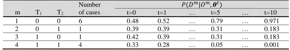
suppose the summarized data is like Table (1).
Table 1. Summarized data set for a Naïve Bayesian network with a binary hidden class node D and two observed binary nodes O=(T1, T2)
m T1 T2
Number of cases
𝑃(𝐷𝑚|𝑂𝑚, 𝜽𝑡)
t=0 t=1 … t=5 … t=10
1 0 0 6 0.48 0.52 … 0.79 … 0.971
2 0 1 1 0.39 0.39 … 0.31 … 0.183
3 1 0 1 0.42 0.39 … 0.31 … 0.183
4 1 1 4 0.33 0.28 … 0.05 … 0.001
Let 𝜃1𝑡 = 𝑃(𝐷 = 1) = 𝜋, 𝜃2𝑡= 𝑃(𝑇1= 1|𝐻 = 1) = 𝑆1, 𝜃3𝑡= 𝑃(𝑇1= 1|𝐻 = 0) = 1 − 𝐶1, 𝜃4𝑡 =
𝑃(𝑇2= 1|𝐻 = 1) = 𝑆2, 𝜃5𝑡 = 𝑃(𝑇2= 1|𝐻 = 0) = 1 − 𝐶2and𝜽𝑡 = (𝜃1𝑡. … . 𝜃5𝑡). 𝜽𝑡’s elements are
theCPTs of our simple network.
Let begin by 𝜽0= (
0.4,0.55,0
.61,0.43,0
.52
). Then we have:𝑃(𝐷1|𝑂1, 𝜽0) = 𝑃(𝐷 = 1|𝑇
1= 𝑇2 = 0, 𝜽0) =
𝑃(𝑇1= 0|𝐷 = 1)𝑃(𝑇2= 0|𝐷 = 1)𝑃(𝐷 = 1)
∑1 𝑃(𝑇1= 0|𝐷 = 𝑑)𝑃(𝑇2= 0|𝐷 = 𝑑)𝑃(𝐷 = 𝑑)
𝑑=0
= 0.450.570.4
0.6 0.48 0.39 0.4 0.57
0.45 = 0.4774
𝑃(𝐷4|𝑂4. 𝜽0) = 𝑃(𝐷 = 1|𝑇
1= 𝑇2= 1. 𝜽0) =
𝑃(𝑇1= 1|𝐷 = 1)𝑃(𝑇2= 1|𝐷 = 1)𝑃(𝐷 = 1)
∑1 𝑃(𝑇1= 1|𝐷 = 𝑑)𝑃(𝑇2 = 1|𝐷 = 𝑑)𝑃(𝐷 = 𝑑)
𝑑=0
= 0.550.430.4
0.6 0.52 0.61 0.4 0.43
0.55 = 0.332
This leads to the expected value of D=1 as:
𝐸(𝐷 = 1) = 60.480.390.4240.33
Now we can re-estimate the parameters for the next iteration: 𝑃̂(𝐷 = 1) =5.01
12 = 0.4175
𝑃̂(𝑇1 = 1|𝐷 = 1) =
𝐸(𝑇1= 1. 𝐷 = 1)
𝐸(𝐷 = 1) =
5
.
01
0
.
347
33
.
0
4
41
.
0
𝑃̂(𝑇1 = 1|𝐷 = 0) =𝐸(𝑇1= 1. 𝐷 = 0)
𝐸(𝐷 = 0) = (12 5.01) 0.466
67 . 0 4 58 . 0
𝑃̂(𝑇2= 1|𝐷 = 1) =𝐸(𝑇2= 1. 𝐷 = 1)
𝐸(𝐷 = 1) =
5
.
01
0
.
34
33
.
0
4
39
.
0
𝑃̂(𝑇2= 1|𝐷 = 0) =𝐸(𝑇2= 1. 𝐷 = 0)
𝐸(𝐷 = 0) = (12 5.01) 0.47
67 . 0 4 61 . 0
189 The above process iterates once more with 𝜽0 replaced by 𝜽1 and leads to 𝜽2 = (
0.42,
0.31,
0.5,
0.3,
0.5
). The iteration process repeats until convergence.K-modes algorithm
The k-modes approach modifies the standard k-means process for clustering categorical data by replacing the Euclidean distance function with the simple matching dissimilarity measure, usingmodes to represent cluster centers and updating modes with the most frequent
categorical valuesin each of iterations of the clustering process (8, 9).
Distance function
To calculate the distance (or dissimilarity) between two objects X and Y described by m categoricalattributes, the distance function in k-modes is defined as:
𝑑(𝑋. 𝑌) = ∑𝑚 𝛿(𝑥𝑖. 𝑦𝑖)
𝑖=1
(5)
where
𝛿(𝑥𝑖. 𝑦𝑖) = {0. 𝑖𝑓𝑥1. 𝑖𝑓𝑥𝑖= 𝑦𝑖 𝑖≠ 𝑦𝑖
Here, xi and yi are the values of attribute j in X
and Y. This function is often referred to as simplematching dissimilarity measure or Hamming distance. The larger the number of mismatches ofcategorical values between X and Y is, the more dissimilar the two objects.
Clustering process
In k-modes clustering, the cluster centers are represented by the vectors of modes of categoricalattributes. To cluster a categorical data set X into k clusters, the k-modes clustering processconsists of the following steps:
Step 1: Randomly select k unique objects as the initial cluster centers (modes).
Step 2: Calculate the distances between each object and the cluster mode; assign the object to thecluster whose center has the shortest distance to the object; repeat this step until all objectsare assigned to clusters.
Step 3: Select a new mode for each cluster and compare it with the previous mode. If different, go back to Step 2; otherwise, stop.
This clustering process minimizes the following k-modes objective function:
𝐹(𝑈. 𝑍) = ∑ ∑ ∑ 𝑢𝑗.𝑙𝑑(𝑥𝑗.𝑖. 𝑧𝑙.𝑖)
𝑚
𝑖=1 𝑛
𝑗=1 𝑘
𝑙=1
Where 𝑈 = [𝑢𝑗.𝑙] is an 𝑛 × 𝑘 partition matrix, 𝑍 = {𝑍1, 𝑍2, … . , 𝑍𝑘} is a set of mode vectors and
the distance function d is defined as in Equation (5).
Performance evaluation
190 nominal coverage probability which is often set
at 0.95, willequal the actual coverage probability. For the simulation study, model's efficiency is evaluated using coverage probability and in the real case of Diabetic retinopathy study, we can
also obtain true positive predictive value (PPV) and negative predictive value (NPV) for each diagnostic test. The formulas for calculating theseaccuracy measures are as below:
𝑃𝑃𝑉 = 𝑃(𝑌𝑖𝑗= 1|𝐷𝑖 = 1)𝑃(𝐷𝑖 = 1)
𝑃(𝑌𝑖𝑗 = 1|𝐷𝑖= 1)𝑃(𝐷𝑖 = 1) + 𝑃(𝑌𝑖𝑗= 1|𝐷𝑖 = 0)𝑃(𝐷𝑖 = 0)
= 𝑆 × 𝜋
𝑆 × 𝜋 + (1 − 𝐶) × (1 − 𝜋)
𝑁𝑃𝑉 = 𝑃(𝑌𝑖𝑗= 0|𝐷𝑖 = 0)𝑃(𝐷𝑖= 0)
𝑃(𝑌𝑖𝑗 = 0|𝐷𝑖 = 0)𝑃(𝐷𝑖 = 0) + 𝑃(𝑌𝑖𝑗= 0|𝐷𝑖 = 1)𝑃(𝐷𝑖 = 1)
= 𝐶 × (1 − 𝜋)
𝐶 × (1 − 𝜋) + (1 − 𝑆) × 𝜋
Simulation study
A simulation study was conducted under the Naïve Bayesian network and the k-modes algorithm, to calculate coverage probability for desired parameters.
Different parameter values for sensitivities and specificities of five tests were considered
in two different scenarios. In each scenario, we pre-defined fixed sets of prevalences and sample sizes. Sample sizes considered in this
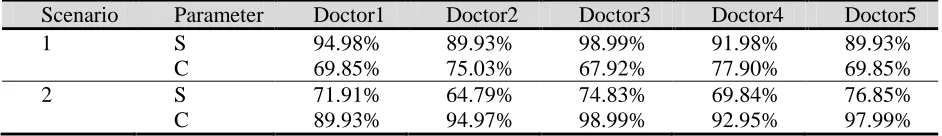
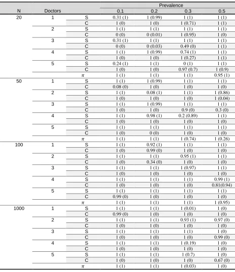
study, are 20, 50, 100 and 1000 and prevalences were set to 0.1, 0.2, 0.3 and 0.5. Under each scenario of sensitivity and specificity, and under each pair of sample sizes and prevalences, we simulated 10000 samples, and calculated the coverage probabilities using boot package in R (16, 17). In the first scenario the sensitivities were set to be high but the specificities to be low, in the second scenario, sensitivities and specificities were set to below and high, respectively (Table (2)).
Table 2. Sensitivity and specificities considered in the simulation study
Scenario Parameter Doctor1 Doctor2 Doctor3 Doctor4 Doctor5
1 S 94.98% 89.93% 98.99% 91.98% 89.93%
C 69.85% 75.03% 67.92% 77.90% 69.85%
2 S 71.91% 64.79% 74.83% 69.84% 76.85%
C 89.93% 94.97% 98.99% 92.95% 97.99%
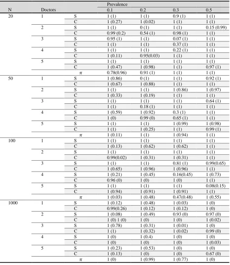
Table (3) demonstrates the coverage probabilities estimated for prevalence, sensitivities and specificities under the first scenario. Coverage probabilities estimated under the second scenario are illustrated in Table (4).
In both scenarios, for each value of prevalence, as the sample size increases the coverage probabilities of Naïve Bayesian network get closer to 1 indicating the rise in the performance of Naïve Bayesian network. For small sample sizes (N=20 and 50), there is an
191 and 4. This indicates the weakness of Naïve
Bayesian network in estimating high sensitivities comparing to high specificities.
Table 3. Coverage probabilities under scenario 1, considering different sample sizes and prevalence values, calculated using Naïve Bayesian network and k-modes algorithm (values in the parentheses)
N Doctors
Prevalence
0.1 0.2 0.3 0.5
20 1 S 1 (1) 1 (1) 0.9 (1) 1 (1)
C 1 (0.27) 1 (0.02) 1 (1) 1 (1)
2 S 1 (1) 0 (1) 1 (1) 0.15 (0.99)
C 0.99 (0.2) 0.54 (1) 0.98 (1) 1 (1)
3 S 0.95 (1) 1 (1) 0.07 (1) 1 (1)
C 1 (1) 1 (1) 0.37 (1) 1 (1)
4 S 1 (1) 1 (1) 0.22 (1) 1 (1)
C 1 (0.11) 0.95(0.03) 1 (1) 1 (1)
5 S 1 (1) 1 (1) 1 (1) 1 (1)
C 1 (0.47) 1 (0.98) 1 (1) 0.97 (1)
𝜋 0.78(0.96) 0.91 (1) 1 (1) 1 (1)
50 1 S 1 (0.86) 0 (1) 1 (1) 0.92 (1)
C 1 (0.67) 1 (0.88) 1 (1) 1 (1)
2 S 1 (1) 1 (1) 1 (0.86) 1 (0.97)
C 1 (0.33) 1 (0.19) 1 (1) 1 (1)
3 S 1 (1) 1 (1) 1 (1) 0.64 (1)
C 1 (1) 0.18 (1) 1 (1) 1 (1)
4 S 1 (0.59) 1 (0.92) 0.3 (1) 1 (1)
C 1 (0) 0.99 (0) 0.65 (1) 1 (1)
5 S 1 (1) 1 (1) 1 (0.99) 1 (0.98)
C 1 (1) 1 (0.25) 1 (1) 0.99 (1)
𝜋 1 (0.11) 1 (1) 1 (0.94) 1 (1)
100 1 S 1 (1) 1 (1) 1 (1) 1 (1)
C 1 (0.13) 1 (0.62) 1 (0.62) 1 (1)
2 S 1 (1) 1 (1) 1 (1) 1 (1)
C 0.99(0.02) 1 (0.31) 1 (0.31) 1 (1)
3 S 1 (1) 1 (1) 0.81 (1) 0.99(0.65)
C 1 (0.65) 1 (0.96) 1 (0.96) 1 (1)
4 S 1 (0.21) 1 (0.45) 0.16(0.45) 1 (0.73)
C 0.96 (0) 1 (0) 1 (0) 1 (1)
5 S 1 (1) 1 (1) 1 (1) 0.08(0.15)
C 1 (0.94) 1 (0.91) 1 (0.91) 1 (1)
𝜋 1 (0.03) 1 (0.48) 0.47(0.48) 1 (0.55)
1000 1 S 1 (0.12) 1 (0.48) 1 (0.03) 1 (0)
C 0.99(0.26) 1 (0.12) 1 (0.12) 1 (0)
2 S 1 (0.08) 1 (0.49) 0.93 (0) 0.97 (0)
C 1 (0) 1 (0) 1 (0) 1 (0) 1 (0.02)
3 S 1 (0.78) 1 (0.31) 1 (0.01) 1 (0)
C 1 (1) 1 (0.32) 1 (0.02) 0.99 (0)
4 S 1 (0) 1 (0.4) 1 (0) 1 (0)
C 1 (0) 1 (0) 1 (0) 1 (0.03)
5 S 1 (0.23) 1 (0.53) 1 (0) 1 (0)
C 1 (0.13) 1 (0) 1 (0) 0.67 (0)
192
Table 4.Coverage probabilities under scenario 2, considering different sample sizes and prevalence values, calculated using Naïve Bayesian network and k-modes algorithm (values in the parentheses)
N Doctors
Prevalence
0.1 0.2 0.3 0.5
20 1 S 0.31 (1) 1 (0.99) 1 (1) 1 (1)
C 1 (0) 1 (0) 1 (0.71) 1 (1)
2 S 1 (1) 1 (1) 1 (1) 1 (1)
C 0 (0) 0 (0.01) 1 (0.95) 1 (0)
3 S 0.31 (1) 1 (1) 1 (1) 1 (1)
C 0 (0) 0 (0.03) 0.49 (0) 1 (1)
4 S 1 (1) 1 (0.99) 0.74 (1) 1 (1)
C 1 (0) 1 (0) 1 (0.27) 1 (1)
5 S 0.24 (1) 1 (1) 0 (1) 1 (1)
C 1 (0) 1 (0) 0.97 (0.7) 1 (0.9)
𝜋 1 (1) 1 (1) 1 (1) 0.95 (1)
50 1 S 1 (1) 1 (0.99) 1 (1) 1 (1)
C 0.08 (0) 1 (0) 1 (0) 1 (0)
2 S 1 (1) 0.08 (1) 1 (1) 1 (0.86)
C 1 (0) 1 (0) 1 (0) 1 (0.04)
3 S 1 (1) 1 (0.99) 1 (1) 1 (1)
C 1 (0) 1 (0) 0.9 (0) 0.3 (0)
4 S 1 (1) 0.98 (1) 0.2 (0.89) 1 (1)
C 1 (0) 1 (0) 1 (0) 1 (0)
5 S 1 (1) 1 (1) 1 (1) 1 (1)
C 1 (0) 0 (0) 1 (0) 1 (0)
𝜋 1 (1) 1 (1) 1 (0.74) 1 (0.26)
100 1 S 1 (1) 0.92 (1) 1 (1) 1 (1)
C 1 (0) 0.99 (0) 1 (0) 1 (0)
2 S 1 (1) 1 (1) 0.95 (1) 1 (1)
C 1 (0) 0.34 (0) 1 (0) 1 (0)
3 S 1 (1) 1 (1) 1 (0.97) 1 (1)
C 1 (0) 1 (0) 1 (0) 1 (0)
4 S 1 (1) 1 (1) 1 (1) 0.99 (1)
C 1 (0) 1 (0) 1 (0) 0.81(0.94)
5 S 1 (1) 1 (1) 1 (1) 1 (1)
C 0.99 (0) 1 (0) 1 (0) 1 (0)
𝜋 1 (1) 1 (1) 1 (1) 1 (0.95)
1000 1 S 1 (1) 1 (1) 1 (0.01) 1 (0)
C 0.99 (0) 1 (0) 1 (0) 1 (0)
2 S 1 (1) 1 (1) 0.93 (1) 0.97 (0)
C 1 (0) 1 (0) 1 (0) 1 (0)
3 S 1 (1) 1 (1) 1 (1) 1 (0)
C 1 (0) 1 (0) 1 (0) 0.99 (0)
4 S 1 (1) 1 (1) 1 (0.19) 1 (0)
C 1 (0) 1 (0) 1 (0) 1 (0)
5 S 1 (1) 1 (1) 1 (0.7) 1 (0)
C 1 (0) 1 (0) 1 (0) 0.67 (0)
𝜋 1 (1) 1 (1) 1 (0.03) 1 (0)
K-modes algorithm is much faster than Naïve Bayesian network, but it has a weakerperformance compared to that of the Naïve Bayesian network. As the number of
193 In the first scenario, where the sensitivities were
set to high levels and specificities to low levels, the k-modes algorithm is more efficient than the second scenario. It can be deduced that it performs well for lower levels of specificities than the higher ones, but nevertheless it is successful in covering sensitivities. It has the best performance for small number of records, prevalence of 0.3 and high level ofsensitivities. Application: Diabetic retinopathy data
Diabetic Retinopathy (DR) is the leading cause of visual loss and blindness among working-agepeople with diabetes in developed and developing countries. One problem in DR
diagnosis is that there is no test which could precisely detect the true disease status.
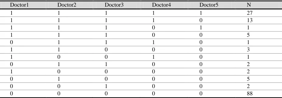
A preliminary study in research center of ophthalmology of Shahid Beheshti University of Medical Science (sbmu) has been conducted to design a network for diagnosis of diabetic retinopathy. The diagnosis of DR was through the fundus photography of 150 patients' retina was screened by 5 doctors. Each doctor, observed the retina photograph of each patient, independently, and made their diagnosis with 0 as no DR and 1 as with DR (Table (5)). In 27 cases, all 5 doctors diagnosed the patients as with DR, and in 88 cases all the doctors randomly agreed on patientswith no DR.
Table 5.Diabetic Retinopathy dataset of 5 doctors for 150 patients
Doctor1 Doctor2 Doctor3 Doctor4 Doctor5 N
1 1 1 1 1 27
1 1 1 1 0 13
1 1 1 0 1 1
1 1 1 0 0 5
0 1 1 1 0 1
1 1 0 0 0 3
1 0 0 1 0 1
0 1 1 0 0 2
1 0 0 0 0 2
0 1 0 0 0 5
0 0 1 0 0 2
0 0 0 0 0 88
The diagnostic test results of 5 doctors using Naïve Bayesian network with the structure of Figure (1), and the k-modes algorithm are applied to obtain the parameters of interest for five different doctors along with their PPV, NPV (Table (6)). As wecan see in Table (6), the two method of Naïve Bayesian network and k-modes
algorithm (values in the parentheses) show a similar level of performances, which is very promising for the k-modesmethod considering its high speed in calculations. Doctors 2 and 3 have the highest and doctor5 lowest sensitivity and doctors 4 and 5 have the highest and doctor 2 has the lowest specificity.
Table 6.The diabetic retinopathy diagnostic test results of 5 doctors for 150 patients using Naïve Bayesian networks and k-modes algorithm (values in the parentheses)
Doctor Sensitivity Specificity PPV NPV
1 0.970(0.979) 0.950 (0.951) 0.900 (0.902) 0.990 (0.990)
2 1.000 (1.000) 0.900 (0.902) 0.830 (0.825) 1.000 (1.000)
3 1.000 (1.000) 0.950 (0.951) 0.910 (0.904) 1.000 (1.000)
4 0.870 (0.872) 1.000 (1.000) 1.000 (1.000) 0.940 (0.944)
5 0.590 (0.596) 1.000 (1.000) 1.000 (1.000) 0.840 (0.843)
194 Doctors 4 and 5 have the best PPV and doctors
2 and 3 together have the best NPV. Also the estimate for the prevalence of the disease is 0.32.
Results
Naïve Bayesian networks and k-modes algorithm were applied to classify patients into diseased and non-diseased categories. In the real case study of diabetic retinopathy, sensitivities for all doctors, except for one, were high enough to detect patients with retinopathy and specificitieswere high to almost perfectly detect non-diseased patients.
In the simulation study, for reasonable values of sensitivities and specificities, as the sample size increases the coverage probabilities of Naïve Bayesian network converges to the pre-specifiedvalue of 95% and higher. But for the k-modes algorithm it decreases to almost zero. In a nutshell, NaïveBayesian network is much more efficient than the k-modes algorithm and also much more time consuming. But there are cases like: small number of records, prevalence of 0.3and high level of sensitivities, that k-modes algorithm achieve better or the same results than Naïve Bayesian network. Also the Naïve Bayesian network's performance seems to be promising for not very large data bases and small prevalence values.
Discussion and Conclusion
In this paper we only investigated a simple case of diagnostic accuracy assessment where a fixed number of doctors assess the same sets of patients. It can be extended to a more complex model, such as repeated assessment of the doctors, assessment of different doctors on different sets of patients. Also the assumption of conditional independence, which can be violated in somecircumstances, should be taken into account for a better estimation of diagnostic criteria.
Conflicts of interests
The authors declare that there is no conflict of interest regarding the publication of this article.
References
1. Gelaye B, Tadesse MG, Williams MA, Fann JR, Stoep AV, Zhou XHA. Assessing validityof a depression screening instrument in the absence of a gold standard. Annals of Epidemiology. 2014;24(7):527-531.
2. Reitsma JB, Rutjes AWS, Khan KS, Coomarasamy A, Bossuyt PM. A review of solutionsfor diagnostic accuracy studies with an imperfect or missing reference standard. Journal ofClinical Epidemiology. 2009;62(8):797-806.
3. van Smeden M, Naaktgeboren CA, Reitsma JB, Moons KGM, de Groot JAH. Latent ClassModels in Diagnostic Studies When There is No Reference Standard: A Systematic Review. American Journal of Epidemiology. 2014;179(4):423-431.
4. Kaufman L, Rousseeuw PJ. Finding Groups in Data: an introduction to cluster analysis.Wiley; 1990.
5. Everitt BS. Cluster Analysis. 3rd ed. John Wiley and Sons Inc; 1993.
6. Lazarsfeld PF, Henry NW. Latent structure analysis. Houghton, Mifflin; 1968.
7. Bartholomew D. Latent Variable Models and Factor Analysis. A Unified Approach. 3rded.Chichester: Wiley; 2011.
8. Huang Z. Extensions to the k-Means Algorithm for Clustering Large Data Sets withCategorical Values. Data Min KnowlDiscov. 1998 Sep;2(3):283-304. 9. Huang Z. A Fast Clustering Algorithm to
Cluster Very Large Categorical Data Sets in DataMining. In: DMKD; 1997.
10. Hui SL, Zhou XH. Evaluation of diagnostic tests without gold standards. Statistical MethodsinMedical Research. 1998;7(4):354-370. PMID: 9871952.
11. Duda RO, Hart PE. Pattern Classification and
Scene Analysis. A Wiley
IntersciencePublication.Wiley; 1973.
195 13. Elidan G, Friedman N. Learning Hidden
Variable Networks: The Information BottleneckApproach. Journal of Machine Learning Research. 2005;6:81-127.
14. Zhang NL. Hierarchical Latent Class Models for Cluster Analysis. J Mach Learn Res. 2004;5:697-723.
15. Dodge Y. The Oxford Dictionary of Statistical Terms. Oxford University Press; 2006.
16. Canty A, Ripley BD. boot: Bootstrap R (S-Plus) Functions; 2017. R package version 1.3-20.