Please cite this article as: R. Mortazavi, S. H. Erfani, An Effective Method for Utility Preserving Social Network Graph Anonymization Based on Mathematical Modeling, International Journal of Engineering (IJE), IJE TRANSACTIONS A: Basics Vol. 31, No. 10, (October 2018) 1624-1632
International Journal of Engineering
J o u r n a l H o m e p a g e : w w w . i j e . i rAn Effective Method for Utility Preserving Social Network Graph Anonymization
Based on Mathematical Modeling
R. Mortazavi*, S. H. Erfani
School of Engineering, Damghan University, Damghan, Iran.
P A P E R I N F O
Paper history: Received 20 March 2018
Received in revised form 25 May 2018 Accepted 17 Auguest 2018
Keywords: Mathematical Modeling Graph Anonymization Graph Modification Social Network Privacy Database Security
A B S T R A C T
In recent years, privacy concerns about social network graph data publishing has increased due to the widespread use of such data for research purposes. This paper addresses the problem of identity disclosure risk of a node assuming that the adversary identifies one of its immediate neighbors in the published data. The related anonymity level of a graph is formulated and a mathematical model is proposed to solve the problem. The application of the method on a number of synthetic and real-world datasets confirms that the method is general and can be used in different contexts to produce superior results in terms of the utility of the anonymized graph.
doi: 10.5829/ije.2018.31.10a.03
1. INTRODUCTION1
The vast dissemination of social networks data for research purposes in recent years has motivated the privacy concerns of individuals. Participants most often expressed privacy concerns about social network services, and the sharing of personal information online left them scared and feeling vulnerable [1]. In fact, in the case of online social networks, there are many reasons such as privacy that restrict datasets to be public which limits the application of interesting machine learning techniques [2]. For instance, in health information dissemination, the shift by health care
providers towards more dynamic methods of
information sharing can be the cause of threat to the privacy of social media platforms [3].
Usually, a social network is represented as a simple graph in which nodes are individuals and edges correspond to a relationship between individuals. Respecting the privacy issues of involving individuals, the owner of the social network has to anonymize the underlying graph before publishing it. Despite the fact that privacy concerns in releasing social network data
*Corresponding Author Email: [email protected] (R. Mortazavi)
have been pinpointed, there is no agreement on the definition of privacy or anonymity that should be used for such data [4].
This paper considers a scenario in which an adversary attempts to re-identify a real-world entity in the graph based on its neighborhood. The main contributions of the paper include the following items: • A new anonymity measure is defined to quantify
the privacy level of a given graph with respect to the anonymity model.
• A mathematical model is proposed to capture a solution that minimizes the information loss of the anonymization process.
• Four different variants of the base mathematical model are proposed by changing its objective function.
• A set of experimental evaluations of the method on multiple synthetic and real-world networks are conducted.
Notation: Let G=(V, E) be a simple graph, in which 𝑉
denotes the set of vertices2 and 𝐸 the set of edges. The
2The terms vertex and node are assumed with the same meaning in this
vertices are referred to by 𝑣𝑖∈ 𝑉 and {Vi, Vj} is used to show an undirected edge between vertices 𝑣𝑖 and 𝑣𝑗.
Assume 𝑛 = |𝑉| denotes the number of vertices. The degree of a vertex 𝑣𝑖∈ 𝑉 is denoted by 𝑑𝑒𝑔(𝑣𝑖) and the
shortest path length between 𝑣𝑖 and 𝑣𝑗 is denoted by
𝑑(𝑣𝑖, 𝑣𝑗). The average of node degrees is also shown as
𝐴𝑉𝐷. Additionally, 𝑁(𝑣) = {𝑢 ∈ 𝑉: {𝑢, 𝑣} ∈ 𝐸} shows neighbors of 𝑣. All notations and abbreviations are defined in Table 1.
Roadmap: The remaining of the paper is organized as follows: Section 2 introduces a number of related works. Section 3 defines the anonymity measure that is used to quantify the privacy and proposes a model to satisfy the related requirement. Section 4 evaluates the proposed method on a number of synthetic and real-world datasets and finally, Section 5 concludes the paper.
2. RELATED WORK
Currently, large amounts of private information are gathered in social networks. It is shown that trivial procedure of removing names or other primary identifiers cannot produce a suitable data for publication [5]. To address the problem, similar to traditional relational data anonymization, some procedures reported in literature [6-9], are proposed. For instance, perturbation-based approaches that randomly insert or delete edges of the graph are considered by Ying and Wu [10]. Hay et al. investigate the potential of structural queries on graphs for the re-identification of vertices and propose an anonymization method based on k-anonymity. Liu et al. [11] introduced k-degree anonymity and Casas Roma et al. [5] presented an efficient algorithm to fulfill the requirement. Feder et al. [4] defined (k, l)-anonymity as a relaxed version of k-anonymity. Based on the definition, a graph G = (V, E) is called (k, l)- anonymous if for every vertex 𝑣 ∈ 𝑉,
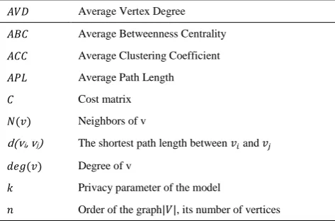
TABLE 1. Abbreviations and notations used in the paper
𝐴𝑉𝐷 Average Vertex Degree
𝐴𝐵𝐶 Average Betweenness Centrality
𝐴𝐶𝐶 Average Clustering Coefficient
𝐴𝑃𝐿 Average Path Length
𝐶 Cost matrix
𝑁(𝑣) Neighbors of v
d(vi, vj) The shortest path length between 𝑣𝑖 and 𝑣𝑗
𝑑𝑒𝑔(𝑣) Degree of v
𝑘 Privacy parameter of the model
𝑛 Order of the graph|𝑉|, its number of vertices
there exists a set of vertices 𝑈 ⊆ 𝑉 not containing 𝑣
such that |𝑈| ≥ 𝑘 and for each 𝑢 ∈ 𝑈, the two vertices
𝑢 and 𝑣 share at least 𝑙 neighbors. The authors devised a random matching algorithm for the special case of (k,1)-anonymity that uses edge addition to produce an anonymous graph. In order to preserve the utility of the produced graph in terms of the number of added edges, the authors consider matching only between problemistic (called deficient) vertices in the original graph. However, Stokes and Torra showed that the original definition of (𝑘, 𝑙)-anonymity suffers from some real-world problems related to privacy of involved vertices and refined the definition.
Definition 1 (Definition 21 of Liu and Terzi [12]). G=(V, E) is (k, l)-anonymous if for any vertex 𝑣 ∈ 𝑉
and for all subset 𝑆 ⊆ 𝑁(𝑣) of cardinality |𝑆| ≤ 𝑙 there are at least 𝑘 distinct vertices {𝑣𝑖}𝑖=1𝑘 such that 𝑆 ⊆
𝑁(𝑣𝑖) for i∈{1,k}.
According to Definition 1 and for the special case of
𝑙 = 1 and 𝑘 ≥ 2, if an adversary identifies a (real) neighbor (𝑣𝑗) of a vertex 𝑣𝑖 in the graph, she would not
be able to re-identify 𝑣𝑖 using 𝑣𝑗 with probability more
than 1/𝑘. The adversary may use different background knowledge such as the degree of the vertex 𝑣𝑗 [5] to
identify it in 𝐺 and then tries to cascade the knowledge to other nodes. Liu and Terzi [12] suggested cloning problemistic vertices, i.e., to insert a number of new vertices with the same neighborhood of the problemistic vertices. However, as stated by Liu and Terzi [12], these fake nodes cause the algorithm to lose its status as an anonymization method. Additionally, an adversary who knows about the anonymization algorithm can re-identify the victim with probability greater than 1/𝑘.
3. THE PROPOSED METHOD
In this paper, we propose a general framework for the
(𝑘, 𝑙)-anonymity problem. The solution uses only edge addition to anonymize the original graph and is formulated as a mixed integer program. According to definition 1, Section 3.1 defines a measure to quantify graph anonymity. Section 3.2 presents the general solution of the problem. Different variants of the model are then introduced in Section 3.3. Finally, Section 3.4 describes the algorithm of the proposed method.
3. 1. The Anonymity of The Original Graphs In this section, we define the anonymity of a graph G=(V, E) based on definition 1.
𝑎𝑛𝑜𝑛𝑦𝑚𝑖𝑡𝑦(𝐺, 𝑘) =
min
𝑖|{𝑣𝑗:𝑣𝑗∈𝑁(𝑣𝑖),𝑑𝑒𝑔(𝑣𝑗)≥𝑘}|
𝑑𝑒𝑔(𝑣𝑖)
Equation (1) calculates the anonymity level of 𝐺 for different values of 𝑘. For each node 𝑣𝑖, the number of
its neighbors with degrees greater than 𝑘 is calculated and is normalized by 𝑑𝑒𝑔(𝑣𝑖). The minimum of the
values for all nodes is considered as the anonymity level for 𝐺. The larger the value, the better the graph is protected against such adversaries.
3. 2. The Mathematical Model The proposed solution attempts to minimize modifications to the original graph while preserving the privacy of nodes with respect to Definition 1. The solution as a mixed integer program contains the following parts:
• Definition of sets: The indexes of vertices 𝑣𝑖∈ 𝑉 in
the graph are saved in 𝐼, i.e., 𝐼 = {1,2, … , 𝑛}. • Fixed parameters and constants: Two parameters 𝑛
and 𝑘 represent the number of vertices, and 𝑘 of the anonymization model, respectively. Additionally, the parameter 𝑐𝑖𝑗 denotes the cost of adding the
edge 𝑒𝑖𝑗 ∉ 𝐸 that connects 𝑣𝑖 and 𝑣𝑗 both in 𝑉. The
cost matrix 𝐶 = [𝑐𝑖𝑗] is symmetric, i.e., 𝑐𝑖𝑗 = 𝑐𝑗𝑖. It
is equal to 0 for connected vertices in the original graph 𝐺, and a positive value for disjoint ones. In order to reduce the size of passed data to the solver, only upper triangular part of 𝐶 is passed to the solver.
• Independent problem variables: The solution consists of vertices to be connected. The binary decision variable 𝑥𝑖𝑗 determines the connectivity of
𝑣i and 𝑣j in the produced anonymized graph, where
𝑥𝑖𝑗 = 1 if the related vertices are to be connected.
In order to decrease the space complexity of the final model we only consider 𝑥𝑖𝑗 for 𝑗 > 𝑖, 𝑖, 𝑗 ∈ 𝐼.
• Objective function: The objective is to minimize the aggregate cost of changes with respect to the original graph, i.e.,
min
𝑥𝑖𝑗 ∑𝑖,𝑗∈𝐼,𝑖<𝑗𝑐𝑖𝑗𝑥𝑖𝑗.
• Constraints: The constraints fall into two categories: edge preserving constraints, and anonymization constraints.
(a)Edge preserving constraints: None of the existing edges in the original graph can be removed, i.e., 𝑥𝑖𝑗 = 1, ∀𝑒𝑖𝑗 ∈ 𝐸. In order to
speed up the calculation, the warm-start strategy is used in which 𝑥𝑖𝑗 = 1 for all of the connected
vertices 𝑣𝑖 and 𝑣𝑗.
(b)Anonymization constraints: These constraints enforce that the minimum degree of each vertex has to be at least 𝑘, i.e.,
∑𝑗<𝑖𝑥𝑗𝑖+ ∑𝑗>𝑖𝑥𝑖𝑗≥ 𝑘∀𝑖 ∈ 𝐼, deg(𝑣𝑖) < 𝑘.
3. 3. The Variants In this work, four different variants of the general mathematical model have been
applied to the original graph. The difference between these variants is in the different cost functions that are supposed to be minimized in the objective function. Specifically, the following models are considered: • Model 1 (M1): In this model, it is assumed that all
edges introduce the same level of destruction to the original graph 𝐺, i.e., 𝑐𝑖𝑗 = 1, ∀𝑖, 𝑗 ∈ 𝐼. Therefore,
the model minimizes the total number of added edges and chooses a random edge when there are different candidates to be added to 𝐺. It is an implementation of the main objective reported in
literature [4] that is used for comparison
throughout the experiments in the paper.• Model 2 (M2): This model tries to add edges that minimize the total length (in the original graph) between connected vertices. This model assumes that connecting two closer vertices is less harmful to the utility, therefore it uses 𝑐𝑖𝑗 = 𝑑(𝑣𝑖, 𝑣𝑗).
• Model 3 (M3): It is interesting to add new edges that minimally change the average path length (𝐴𝑃𝐿) of
G
as an important property of the graph. This model tries to add edges that decrease 𝐴𝑃𝐿minimally. It is hard to calculate the amount of change in 𝐴𝑃𝐿 for a large number of sets of candidate edges since these edges reinforce the value for other edges. Therefore, the model approximates the total costs of a number of newly added edges by aggregating their individual effects on 𝐴𝑃𝐿. More precisely, if 𝑐𝑖𝑗 is the amount of
change in the 𝐴𝑃𝐿 of the original graph by addition of 𝑒𝑖𝑗 to 𝐺, the total value of the change in the 𝐴𝑃𝐿
for a set of new edges 𝐸′⊂ 𝑉 × 𝑉\𝐸 is
approximated by ∑𝑒𝑖𝑗∈𝐸′𝑐𝑖𝑗.
• Model 4 (M4): Inspired from [13], added edges in this model are chosen to connect similar vertices in terms of the overlap of their neighbors. This model assumes that the cost of connecting two disjoint vertices with very different neighbors is more than the cost of connecting two similar vertices with some more overlap in the neighborhoods. For this model 𝑐𝑖𝑗 = |𝑁(𝑣𝑖) ∪ 𝑁(𝑣𝑗)|/|𝑁(𝑣𝑖) ∩ 𝑁(𝑣𝑗)| is
used.
3. 4. The Algorithms The algorithm of the proposed method is given in Algorithm 1. The function accepts the adjacency matrix 𝑀 of the graph 𝐺, selected variant of the model 𝑉𝑎𝑟, and the privacy parameter 𝑘
as input and produces the anonymized graph 𝐺𝑘. In the
first step, the Compute Cost function is called to compute 𝐶 (Line 1). Next, the optimization problem is solved to obtain the modified adjacency matrix 𝑀′ (Line 2). In Line 3, the anonymized graph 𝐺𝑘 is generated
based on 𝑀′. Finally, 𝐺
𝑘 is returned (Line 4). Algorithm
adjacency matrix 𝑀 and the selected model variant 𝑉𝑎𝑟. Based on the selected model variant, a different cost matrix 𝐶 has to be computed as output. If M1 is chosen,
𝑐𝑖𝑗 will be equal to 0 when 𝑣𝑖 is connected to 𝑣𝑗 in the
original graph 𝐺, otherwise it is set to 1, i.e., 𝑐𝑖𝑗= 1 −
𝑀[𝑖, 𝑗]. This is computed in Line 1. For the case of M4 (Line 2), the cost matrix can be computed efficiently using bitwise operators or and and for the union and intersection functions, respectively. The size function also computes the number of 1st of its operand (Line 3). It is notable that a very small value 𝜖 is added to the denominator to prevent arithmetic errors. The other two options for 𝑉𝑎𝑟, i.e., M2 and M3 are considered in Lines 4-16. In Line 5, the graph-theoretic shortest distance between all nodes are computed using the Floyd-Warshall algorithm [14]. For M2, the computed distances 𝑑𝑖𝑗 minus 1 are returned3 as 𝑐𝑖𝑗(Line 6). For
M3, the function calculates the average value of shortest paths and saves it in 𝐴𝑃𝐿 (Line 8). Then, in the following steps for each 𝑖, 𝑗, the value of 𝑐𝑖𝑗 is
calculated. If 𝑣𝑖 is connected to 𝑣𝑗(𝑖 ≠ 𝑗), 𝑐𝑖𝑗 is set to 0
(Line 11). Otherwise, these vertices are connected temporarily (Line 14) and the new 𝐴𝑃𝐿 is computed (Line 15) and saved in 𝐴𝑃𝐿′ (Line 16). The difference
between 𝐴𝑃𝐿 and 𝐴𝑃𝐿′ is stored in 𝑐
𝑖𝑗 (Line 17).
Finally, the cost function 𝐶 is returned (Line 18).
ALGORITHM 1. Generating the anonymized graph 𝐺𝑘
Input:𝑀 (adjacency matrix of 𝐺), 𝑉𝑎𝑟 (model variant),𝑘
(privacy parameter)
Output: Anonymized graph 𝐺𝑘
Function 𝐺𝑘=AnonymizeGraph(𝑀, 𝑉𝑎𝑟, 𝑘)
1 𝐶=ComputeCost(𝑀, 𝑉𝑎𝑟) // Algorithm 2
2 Solve the optimization problem introduced in Section 3.2 to obtain 𝑀′= [𝑥
𝑖𝑗]
3 𝐺𝑘 = graph(𝑀′)
4 Return 𝐺𝑘
END Function
ALGORITHM 2. Computation of the cost matrix
Input:𝑀 (adjacency matrix of 𝐺), 𝑉𝑎𝑟 (model variant)
Output: The cost matrix 𝐶 Function𝐶=ComputeCost(𝑀,𝑉𝑎𝑟)
1 If𝑉𝑎𝑟 ==M1 Return Ones(𝑛, 𝑛)-𝑀
2 Elseif𝑉𝑎𝑟 ==M4
3 Return 𝐶 = [𝑐𝑖𝑗] where
𝑐𝑖𝑗=Size(Or(𝑀[𝑖, : ], 𝑀[𝑗, : ])) /
(𝜖+Size(And((𝑀[𝑖, : ], 𝑀[𝑗, : ]))) ∀𝑖, 𝑗 ∈ 𝐼
4 Else // M2 or M3
5 𝐷 = [𝑑𝑖𝑗] =Floyd-Warshall(𝑀)
6 If 𝑉𝑎𝑟 ==M2 Return𝐷 − 1
7 Else // M3
8 𝐴𝑃𝐿 =average(𝐷)
3If 𝑣
𝑖 is connected to 𝑣𝑗 (𝑖 ≠ 𝑗) then 𝑑𝑖𝑗= 1. So, 𝑐𝑖𝑗= 𝑑𝑖𝑗− 1 = 0 is considered.
9 Foreach 𝑖, 𝑗 ∈ 𝐼
10 If𝑀[𝑖, 𝑗] == 1
11 𝑐𝑖𝑗= 0
12 Else
13 𝑀′= 𝑀
14 𝑀′[𝑖, 𝑗] = 𝑀′[𝑗, 𝑖] = 1
15 𝐷′= Floyd-Warshall(𝑀′)
16 𝐴𝑃𝐿′=average(𝐷′)
17 𝑐𝑖𝑗= 𝐴𝑃𝐿 − 𝐴𝑃𝐿′
18 Return 𝐶
End Function
4. EXPERIMENTAL EVALUATIONS
In this section, different experiments are conducted to evaluate the efficacy of the proposed method. In all experiments, a PC with Intel Core 2 Duo 3.6 GHz CPU, 16 GB of main memory and Windows 10 operating system is used. The CPLEX optimization engine is used to solve the mathematical problem. Section 4.1 introduces the datasets. Section 4.2 evaluates the risk of the original datasets based on Equation (1). Section 4.3 reports the usefulness of the anonymized graphs based on different utility measures. At the end of this section, execution times are reported in Section 4.4.
4. 1. The Graph Datasets The proposed method is applied to two synthetic and two real-world datasets to observe its performance in different situations. The synthetic datasets are summarized as follows:
• SF50 and SF500: Two scale-free datasets based on Barabasi’s model. These graphs are connected graphs where vertex degrees are drawn from a power-law distribution similar to real-world social networks. The datasets are generated using the tool introduced in [15].
• RA82: A random network based on Erdos-Renyi model in which vertices are connected based on probability 𝑝 = 0.03.
Additionally, three real-world datasets are tested to assess our method in different topologies. The first two datasets are also used in [13].
• PolBooks: A network of books about US politics sold by Amazon.com. Edges in the network show the frequent purchasing of buyers. The data is compiled by V. Krebs (www.orgnet.com).
• Football: the network of American football games between Division IA colleges during regular season Fall 2000, as compiled by Girvan and Newman [16].
• Dwt1005: An undirected graph from Everstine’s collection that is included in the Harwell-Boeing database4.
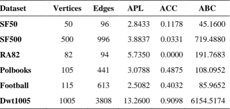
Structural properties of the graphs are given in Table 2. For each graph, the Average Path Length (APL), the Average Clustering Coefficient (ACC), and the Average Betweenness Centrality (ABC) are reported. The APL is a concept in the network topology that is defined as the average number of steps along the shortest paths for all possible pairs of network nodes. It is a measure of the efficiency of information or mass transport on a network5. The ACC is the average of local clustering coefficients of graph nodes. The measure for a node quantifies how close its neighbors are to being a clique and determines whether a graph is a small-world network [17]. Moreover, ABC is the average of betweenness centrality of all nodes. The measure for each node captures the number of shortest paths in the graph passing through the node6.
4. 2. The Anonymity Measure Table 3 shows the measure for the synthetic and real-world graphs introduced in section 3.1. The results confirm that the anonymity of graph diminishes very fast when 𝑘
increases. For instance, for 𝑘 = 4 in Polbooks, there is at least one node 𝑣 for which the degree of half of its neighbors is lower than 4. Therefore, if an adversary identifies one of the neighbors randomly, the probability
to limit𝒗 in a group with lower than 4 members is more
than 0.5.
TABLE 2. Structural properties of Synthetic and Real-world graphs
Dataset Vertices Edges APL ACC ABC
SF50 50 96 2.8433 0.1178 45.1600
SF500 500 996 3.8837 0.0331 719.4880
RA82 82 94 5.7350 0.0000 191.7683
Polbooks 105 441 3.0788 0.4875 108.0952
Football 115 613 2.5082 0.4032 85.9652
Dwt1005 1005 3808 13.2600 0.9098 6154.5174
TABLE 3. Anonymity of different datasets based on Equation (1)
𝒌 = 𝟑 4 5 6 7 8 9 10 11 12 13
SF50 1.00 0.40 0.20 0.00 0.00 0.00 0.00 0.00 0.00 0.00 0.00
SF500 0.33 0.00 0.00 0.00 0.00 0.00 0.00 0.00 0.00 0.00 0.00
RA82 0.33 0.00 0.00 0.00 0.00 0.00 0.00 0.00 0.00 0.00 0.00
Polbooks 1.00 0.67 0.50 0.50 0.25 0.00 0.00 0.00 0.00 0.00 0.00
Football 0.82 0.82 0.82 0.82 0.82 0.82 0.82 0.67 0.60 0.36 0.00
Dwt1005 1.00 1.00 0.67 0.33 0.17 0.00 0.00 0.00 0.00 0.00 0.00
5 https://en.wikipedia.org/wiki/Average_path_length
6 https://en.wikipedia.org/wiki/Betweenness_centrality
Generally, the results show the importance of considering the anonymization process, especially for
𝒌 ≥ 𝟒 with respect to Definition 1 for different datasets.
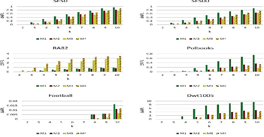
4. 3. The Utility of Anonymized Graphs This section reports the amount of error introduced in the anonymized graph after applying the proposed method. The performance measures are based on the
𝐴𝑉𝐷, 𝐴𝑃𝐿, 𝐴𝐶𝐶, and 𝐴𝐵𝐶 that are defined in Section 4.1. For example, Δ𝐴𝑃𝐿 = |𝐴𝑃𝐿2− 𝐴𝑃𝐿1| where
𝐴𝑃𝐿1 and 𝐴𝑃𝐿2 are the 𝐴𝑃𝐿 of the original and
anonymized graphs, respectively. Other measures are defined similarly. The lower the value, the better the anonymization procedure and the anonymized graph is more similar to the original one. Figures 1-4 show these quantities for different datasets and models. The results confirm for all models that when 𝑘 increases, all error measures increase. For instance, 𝛥𝐴𝑃𝐿 = 0.1241 in SF50 for 𝑘 = 3 and M1, while the value increases to
𝛥𝐴𝑃𝐿 = 0.4604 for 𝑘 = 5. Similarly, 𝛥𝐴𝑉𝐷 = 0.572
in SF500 for 𝑘 = 3 and M3, while the error reaches
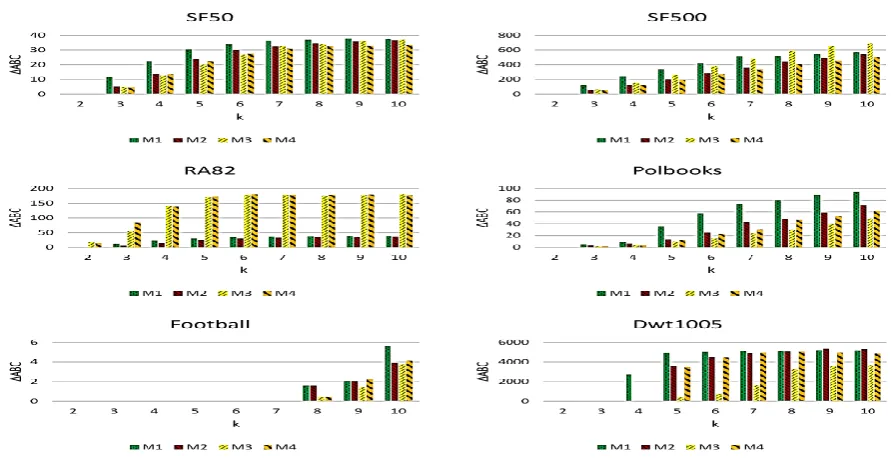
𝛥𝐴𝑉𝐷 = 6.86 for 𝑘 = 10. Figure 1 shows that M1 is always successful to reach the best 𝛥𝐴𝑉𝐷, since the measure is minimized when the number of added edges is minimized, which is the main task of M1 [4]. The results in Figure 2 indicate that in most cases, M3 achieves the best 𝛥𝐴𝑃𝐿. This is rational since the weights in M3 represent the cost related to 𝐴𝑃𝐿, therefore edges with smaller costs have more priority to be added to the solution of the model. For instance, in Dwt1005, 𝛥𝐴𝑃𝐿 = 9.5045 for M1 and 𝑘 = 10, while the quantity is 𝛥𝐴𝑃𝐿 = 1.1955 for M3 which means a significant improvement in compare with literature [4]. Figure 3 shows that in all cases except for the Polbooks and Dwt1005, M1 produces a more useful graph in terms of Δ𝐴𝐶𝐶. This confirms that 𝐴𝐶𝐶 is more sensitive to the number of added edges than the way they are added. Finally, Figure 4 validates again the claim, i.e., a model with the minimum number of added edges does not necessarily result in the best utility for the anonymized graph. For SF50, in 𝑘 ≤ 6, M3 usually produces the lowest errors, while for 𝑘 > 6, M4 achieves the most useful datasets in terms of 𝛥𝐴𝐵𝐶. Interestingly, M3 is also the winner in Polbooks, Football and Dwt1005 graphs. However, for RA82, M2 has the best performancein all cases. This may be related to the structure of RA82, which is a very sparse graph (its initial density is lower than 0.03) while other graphs are at least twice denser than RA82. As the figure illustrates, RA82 is more sensitive than the other three graphs in terms of 𝛥𝐴𝐵𝐶. Similar comparison based on these measures confirm that RA82 is more sensitive to the anonymization procedure. For instance,
during anonymization for the proposed method which is based on edge addition. Therefore, it is suggested to social network owners to allow their network grows to a minimum threshold (for example in terms of its density), and then attempt to apply anonymization procedure on it.
4. 4. Execution Time In this section, the running time of experiments are reported. The main time-consuming tasks consist of solving the optimization problem and computing the cost matrix. Other computations in each separate experiment require less than 2 seconds and are ignored.
Figure 1. The value of ∆𝐴𝑉𝐷 for different datasets and models in 𝑘 = 2. . .10
Figure 3. The value of ∆𝐴𝐶𝐶 for different datasets and models in 𝑘 = 2. . .10
Figure 4. The value of ∆𝐴𝐵𝐶 for different datasets and models in 𝑘 = 2. . .10
Table 4 shows the time required to solve the problem for each dataset and model. The results confirm that in most cases, the problem can be solved in a reasonable time. There may be some cases in which the engine requires a considerable time to produce the optimal solution. It is notable that graph anonymization task is usually considered as an offline procedure. If solving time matters, the optimization engine can be tuned to stop if a near to optimal solution is achieved using the
gap>07.
The other time-consuming task is the Compute Cost function in which the cost matrix 𝐶 is computed. This task is independent of the privacy parameter 𝑘. Table 5 shows the execution time of the function for different datasets and model variants.
TABLE 4. The average solve time (in second) for each dataset and model variant
Dataset M1 M2 M3 M4
SF50 0.23 0.23 0.28 0.22
SF500 3.25 2.85 3.09 339.89
RA82 0.27 0.26 0.26 161.55
Polbooks 0.24 0.25 0.25 0.24
Football 0.21 0.20 0.20 0.20
Dwt1005 6.38 6.25 5.74 5.47
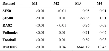
TABLE 5. Execution time of the Compute Cost function (in second) for each dataset and model variant
Dataset M1 M2 M3 M4
SF50 <0.01 <0.01 0.05 0.01
SF500 <0.01 0.01 368.85 1.31
RA82 <0.01 <0.01 0.26 0.02
Polbooks <0.01 0.01 0.71 0.02
Football <0.01 0.01 0.89 0.03
Dwt1005 <0.01 0.04 6641.12 13.45
These running times are almost negligible with respect to the solving time of the optimization problem except for the case of M3. In this case, it is required to call Floyd-Warshall multiple times, so the execution time gets considerable especially for large graphs.
5. CONCLUSIONS
This paper realizes a procedure for graph anonymization. The adversary is assumed to be able to identify a neighbor of a victim node. Regarding this attack model, an anonymity measure is defined. It is shown that the measure decreases sharply when the anonymity parameter increases slightly. A general mathematical model is proposed to increase the anonymity measure using edge addition. Four different variants of the general model are proposed. The procedures are evaluated on different synthetic and real-world graphs. The results show that trying to minimize the number of added edges is not usually a good objective to produce a useful anonymized graph. Additionally, the results show that highly sparse graphs are very sensitive to different utility measures. Evaluating the proposed method for other general graph utility measures is considered to be accomplished as a future work. Moreover, it is interesting to devise some heuristics to anonymize larger social networks [18] without using mixed integer programming approach.
6. REFERENCES
1. Asadi Saeed Abad, F. and Hamidi, H., "An Architecture for Security and Protection of Big Data", International Journal of Engineering, Vol. 30, No. 10, (2017), 1479-1486.
2. Hemati, H., Ghasemzadeh, M. and Meinel, C., "A Hybrid Machine Learning Method for Intrusion Detection",
International Journal of Engineering, Transactions C: Aspects, Vol. 29, No. 9, (2016), 1242-1246.
3. Sharma, P. and Kaur, P. D., "Effectiveness of web-based social sensing in health information dissemination-A review", Telematics and Informatics, Vol. 34, No. 1, (2017), 194–219.
4. Feder, T., Nabar, S. U. and Terzi, E., "Anonymizing graphs",CoRR, abs/0810.5578, (2008).
5. Casas-Roma, J., Herrera-Joancomartí, J. and Torra, V., "k-Degree anonymity and edge selection: improving data utility in large networks", Knowledge and Information Systems, Vol. 50, No. 2, (2017), 447–474.
6. Sweeney, L., "k-anonymity: A model for protecting privacy",
International Journal of Uncertainty, Fuzziness and Knowledge-Based Systems, Vol. 10, No. 5, (2002), 557–570. 7. Mortazavi, R. and Jalili, S., "Enhancing aggregation phase of
microaggregation methods for interval disclosure risk minimization", Data Mining and Knowledge Discovery, Vol. 30, No. 3, (2016), 605–639.
8. Salari, M., Jalili, S. and Mortazavi, R., "TBM, a transformation based method for microaggregation of large volume mixed data", Data Mining and Knowledge Discovery, Vol. 31, No. 1, (2017), 65–91.
9. Machanavajjhala, A., Kifer, D., Gehrke, J. and Venkitasubramaniam, M., "L-diversity: Privacy beyond k-anonymity", ACM Transaction on Knowledge Discovery from Data (TKDD), Vol. 1, No. 1, (2007), 1–52.
10. Ying, X. and Wu, X., "Randomizing social networks: a spectrum preserving approach", in Proceedings of the 2008 SIAM International Conference on Data Mining, SIAM, (2008), 739– 750.
11. Liu, K. and Terzi, E., "Towards identity anonymization on graphs", in Proceedings of the 2008 ACM SIGMOD international conference on Management of data, ACM, (2008), 93–106.
12. Stokes, K. and Torra, V., "Reidentification and k-anonymity: A model for disclosure risk in graphs", Soft Computing, Vol. 16, No. 10, (2012), 1657–1670.
13. Ninggal, M. I. H. and Abawajy, J. H., "Utility-aware social network graph anonymization", Journal of Network and Computer Applications, Vol. 56, (2015), 137–148.
14. Floyd, R. W., "Algorithm 97: Shortest Path", Communications
of the ACM, Vol. 5, No. 6, (June 1962), 345.
doi>10.1145/367766.368168
15. Hadian, A. and Nobari, S., Minaei-Bidgoli, B., Qu, Q., "Roll: Fast in-memory generation of gigantic scale-free networks", in Proceedings of the 2016 International Conference on Management of Data, SIGMOD ’16, ACM, New York, NY, USA, (2016), 1829–1842.
16. Girvan, M. and Newman, M. E., "Community structure in social and biological networks", in Proceedings of the national academy of sciences, Vol. 99, No. 12, (2002), 7821–7826. 17. Watts, D. J. and Strogatz, S. H., "Collective dynamics of
An Effective Method for Utility Preserving Social Network Graph Anonymization
Based on Mathematical Modeling
R. Mortazavi, S. H. Erfani
School of Engineering, Damghan University, Damghan, Iran.
P A P E R I N F O
Paper history: Received 20 March 2018
Received in revised form 25 May 2018 Accepted 17 Auguest 2018
Keywords: Mathematical Modeling Graph Anonymization Graph Modification Social Network Privacy Database Security
هدیکچ
لاس رد هداد راشتنا زا ناربراک ینارگن ،ریخا یاه هکبش یاه
یارب تاعلاطا نیا زا هدرتسگ هدافتسا هب هجوت اب یعامتجا یاه
تاعلاطا مجاهم هکنیا ضرف اب هکبش رد هرگ کی هسانش یاشفا رطخ هب هلاقم نیا رد .تسا هتفای شیازفا یشهوژپ فادها ی هیاسمه زا یک یم هتخادرپ ،دراد رایتخا رد ار هرگ نآ لصفلاب یاه
یب حطس ادتبا .دوش نیا ساسا رب هکبش فارگ کی یمان
لومرف رطخ یدنب یم هئارا رطخ نیا لح یارب یضایر لدم کی همادا رد و هدش یدادعت یور رب قوف شور زا هدافتسا .دوش
هداد هعومجم زا ناشن یعقاو و یعونصم یاه
یم هک تسا قوف شور تیمومع هدنهد جیاتن فلتخم یاهدربراک رد دناوت
هداد یدنمدوس بسح رب ار یبسانم یب یاه
مان هب هدش یزاس .دروآ تسد