Firm Specific Risk and Return: Quantile Regression Application

Firm Specific Risk and Return: Quantile Regression Application

Maryam Davallou

Department of Finace, Faculty of Management and Accounting Shahid Beheshti University, Tehran

[email protected]

Abstract

The present study aims at investigating the relationship between firm specific risk and stock return using cross-sectional quantile regression. In order to study the power of firm specific risk in explaining cross-sectional return, a combination of Fama-Macbeth (1973) model and quantile regression is used. To this aim, a sample of 270 firms listed in Tehran Stock Exchange during 1999-2010 was investigated. The results revealed that the relationship between firm specific risk and stock return is significantly affected by the quantile so that the direction of changes in low quantiles is negative, and in high quantiles, is positive. Moreover, using the specific risk measure based on return’s standard deviation, the interactive effects of industry and the fourth moment lead to removal of this relationship. One can attribute this relation to the mutual effect of industry and kurtosis. However, using measures based factor models, industry and kurtosis cannot eliminate the explanatory power of specific risk.

Keywords: Quantile Regression, Asset Pricing, Firm Specific Risk, Stock Return.

JEL Classification: G12, C21.

1. Introduction

Irrelevance of firm specific risk (FSR) in asset pricing due to the possibility of its removal by diversification is one of the major assumptions of classical finance. Despite market barriers like transaction costs, it can be theoretically indicated that it is not possible to form a diversified portfolio and completely remove FSR, as transaction costs prevent investors from accessing complete information about the features of all securities in the market. Hence, investors often invest upon limited securities expecting to get a positive return on FSR (Merton, 1987). The importance of FSR in explaining the changes of asset return owes to the studies of Ang et al. (2006) for indicating the negative relationship between FSR and return (Ang et al., 2006). In this way, the bases of classical finance and Merton’s theory (1987) are challenged. The emergence of the reverse relationship between FSR and return has recently changed into one of the challenging areas of finance. More empirical findings confirming this relationship belong to developed stock markets, which add to the ambiguity of this issue in developing markets. It can be argued that this relationship is a phenomenon specific to developed markets and it must be generalized to other markets, particularly less developed ones, with care. Investigating the relationship gains importance when empirical evidence of developed markets is extremely contradictory; while some studies consider the direction of changes of FSR and return as positive, others emphasize a negative relationship or even no relationship between them.

One of the common methods for investigating FSR and return is using ordinary least squares (OLS) regression. As long as error terms are normally distributed, estimation of OLS will be the unbiased estimation of regression coefficients, but if error terms have long tails, the estimates may not be so efficient. In this condition, some outliers are expected. When there are outliers, OLS is not an appropriate method. Hence, other estimation methods are presented which are not sensitive to the outliers. Quantile regression is one of such methods. The main motivation underlying quantile regression is its innate power against outliers in the response variable. While OLS is sensitive to a remote observation, in quantile regression the effect of such observations on parameter estimation is limited (Fatahi & Gerami, 2004).

stock return that are expected to gain average return. Quantile regression is a powerful tool which describes the whole distribution of dependent variable. Instead of describing the tendency of the average effect of firm specific volatility as least squares regression, quantile regression is able to indicate the effect of FSR on each of probable values of cross-sectional return. Also, Fama-Macbeth regression (1973), though considered as a kind of standard methodology in finance, has been criticized for low power and susceptibility to error of estimation, and lack of dependence and homoscedasticity between cross-sectional returns. When there are errors in variables and hetroscedasticity, quantile regression is more powerful than least squares regression. Quantile regression analysis of cross-sectional return reduces some statistical problems present in Fama-Macbeth regression (Wan & Xiao, 2014). Therefore, the main goal of this study is to investigate FSR and cross-sectional return in Tehran Stock Market using a combination of quantile regression and Fama-Macbeth model (1973).

2. Background

stock and cross-sectional return is statistically insignificant. The findings indicate that if the price changes are volatile, there would be no relationship between risk and return (Li, 2009). Chiang and Li (2012) studied the relationship between risk and return in U.S. market using weighted least squares and quantile regressions. Weighted least squares regression confirmed the positive relationship between excess return and expected risk. However, quantile regression revealed that the relationship between risk and return changes from negative to positive by increasing return quantile, and the positive relation of risk and return is valid only in high quantiles (Chiang & Li, 2012). Meligkotsidou et al. (2012) used quantile regression for predicting equity. Using quantile regression and fixed and variable weight patterns over time, he explored the distribution data of each predictor. The findings indicated that predictions based on this method are statistically and economically more significant than both methods of mean historical basis and mixed regression approaches (Meligkotsidou et al. 2012).

Wan & Xiao (2014) argues that EGARCH estimates of FSR are associated with significant estimation errors, and the results of studies conducted on its basis are seriously questioned. The assumption of normal distribution in EGARCH model on single security is unrealistic. This assumption is not confirmed at the 5% level of significance in over 90% of securities purchased in NYSE, NASDAQ, and AMEX. Hence, within the framework of “qunatile regression”, they use a new method for estimating the relationship between FSR and return as it does not require consideration of any assumption on the distribution of asset return. They believe that ignoring skewness of the distribution in FSR pricing causes the relationship to be positive in some cases and negative in some other (Wan & Xiao, 2014).

appears that the inverse relationship between FSR and return results from 35% securities whose risk ranking has changed throughout successive months (Saryal, 2009).

3. Methodology

The statistical sample of the present study consisted of all firms accepted in Tehran Stock Market during 1999-2010. The sample consisted of all firms of the population except banks, leasing, investment, and holding companies due to their different asset and capital structure, as well as firms whose book value of equity was negative in the year t-1. Also, firms which did not meet the minimum trading limits posed for relatively fixing the consequences of “nonsynchronous trading”, i.e. 15, 22, and 30 days in the quarters ending in April, July, October and January, were excluded.

Data used in this study were collected from the Securities and Exchange Organization, Tehran Stock Exchange, and Tehran Securities Exchange Technology Services Company.

3.1.Operational definition of variables

The variables of this study are defined and measured as presented in Table 1:

Table 1. Measurement of Research Variables 𝒓𝐢= 𝐥𝐧𝐏_𝐏𝟐

𝟏, where 𝐏𝟏 and 𝐏𝟐 are adjusted for increasing capital and dividend.

Stock return

On the basis of CAPM modified based on Dimson’s model (1979): time series regression of market return and stock return in each quarterly time interval is estimated based on the relation (1):

Rit= αit+ βit−1Rmt−1+ βitRmt+ βit+1Rmt+1+ εit (1)

Where, Rit is the excess return of stock i in day t, Rmt is the excess return

of market in day t, and Rmt−1 and Rmt+1 are the excess return of market in

days t-1 and t+1, and εi,t is the residual of day t. Unsystematic quarterly

volatility is calculated by multiplying the standard deviation of daily residual in the square trading days of the quarter.

Firm Specific

On the basis of three-factor model: following Ang et al. (2006), equation (2) is estimated during every 47 quarters of 1999 to 2010 for each sock. Daily data is used for estimating equation (2):

(2)

Ri,t− rf,t= αi,t+ βi,t(Rm,t− rf,t) + si,tSMBt+ hi,tHMLt+ εi,t

Where, Ri,t is daily excess return of stock i, Rm,t is daily excess return of

market, rf,t is risk-free rate, and εi,t is daily residual. Unsystematic

quarterly volatility is calculated by multiplying the standard deviation of daily residual in the square trading days of the quarter.

On the basis of Carhart four-factor model: residual standard deviation of Carhart’s four-factor model is used for measuring FSR:

Ri,t− rf,t= αi,t+ βi,t(Rm,t− rf,t) + si,tSMBt+ hi,tHMLt+ wi,tWMLt+ εi,t (3)

Where, WMLt is the difference of returns of winner and loser portfolios.

Calculated on the basis of natural logarithm of firm’s market value. Size

Like Amihood (2002), liquidity is defined as follows:

ILIQi,t= |ri,d| Vol⁄ i,t (4)

Voli,t and |ri,d| are respectively dollar value of transactions and absolute

value of stock return in day t. Liquidity

Is calculated based on market model and by modifying Dimson’s model (1979) with a leaded and lagged market return for reducing the consequence of nonsynchronous trading.

Beta

The ratio of trading value to the number of outstanding share. Turnover

Risk-free return rate is equivalent to participant security rate. Risk-free

return

If the firm under study belongs to a specific industry, dummy variable of that industry accepts 1, otherwise it accepts 0.

Industry

Cumulative return of t-3 to t-9 time period. Momentum

Percentage of legal persons’ ownership is used as an approximation of the percentage of institutional ownership.

Institutional ownership

A three-month time break in the calculation of momentum is considered for avoiding the correlation of momentum and FSR resulting from calculation time overlap, as FSR is calculated during a three-month period ending in specific times.

3.2. Quantile regression

𝑌𝑖 = 𝛼 + 𝛽𝑋𝑖+ 𝜀𝑖 (5)

In equation (5), 𝜀𝑖 is the random variable, 𝛼 and 𝛽 are unknown

parameters and 𝑋𝑖 is the known value of explanatory variables. If

𝐸(𝜀𝑖) = 0, equation (5) can be rewritten as follows:

𝐸(𝑌𝑖) = 𝛼 + 𝛽𝑋𝑖 (6)

𝐸(𝑌_𝑖) is called conditional mean of random variable. Thus, according to equation (6), distribution means of Y in different levels of explanatory variable are located along a straight line. In other words, Y random variable has a distribution whose means are on a straight line. Since mean is one of the measures of central tendency, specifying it alone would not present complete information about the form of distribution. In this respect, ordinary regression cannot offer much information about the distribution of random variable under study at various levels of explanatory variable, too. Quantiles are other criteria of distribution which, “together”, can depict a more complete distribution form. For example, if higher deciles are more distant from each other and lower deciles are close to each other, the distribution will skew to the right. Quantile regression model is used for conditional qunatiles as ordinary regression is used for conditional mean. In order to offer an accurate definition of quantile regression of 𝜃 ∈ (0,1), consider the equation (5) with condition 𝜀𝑖~𝐹(0) (function F refers to a given distribution). The

objective is to find a model depicting the relationship between the first quantile (not the mean) of distribution Y and variable X. The model for 𝜃 ∈ (0,1)th quantile of variable Y indicated by 𝑄𝜃(𝑌|𝑋𝑖) is as follows:

𝑄_𝜃(𝑌|𝑋𝑖) = 𝛼 + 𝛽𝑋𝑖+ 𝐹−1(𝜃) (7)

The above function for different 𝜃 ∈ (0,1) will give a set of parallel lines with different Y-intercepts. If F(0) is the normal distribution (or any other symmetric distribution), for 𝜃 = 0.5, equation (6) would equal equation (7). For general explanation of quantile regression model, suppose 𝑌𝑖 = 𝑋́ 𝛽𝑖 𝜃+ 𝜀𝜃𝑖 ,

𝑄_𝜃(𝑌|𝑋́ ) = 𝑋_𝑖 ́ 𝛽_{𝑖 𝜃} 𝑖 = 1,2, … , 𝑛, (8)

Where, 𝑋́ = (1, Xi i1, … , Xik) and βθ = (β0, 𝛽1, … , 𝛽𝑘) are vectors of

𝑄_𝜃(𝑌|𝑋𝑖) is the conditional 𝜃 ∈ (0,1)𝑡ℎ qunatile of distribution Y. Thus,

𝑄_𝜃(𝜀𝜃|𝑋𝑖) = 0. Equation (8) with mentioned conditions is called linear

regression model of θth quantile. Estimation of the parameters of the ordinary regression model is based on minimizing the squares of model deviations which is called least squares method. In this method, the regression line is estimated in order for the distance of points from this line to be minimized. In quantile regression, despite the ordinary regression, minimization of sum of weighted deviations absolute value is used for parameter estimation which is called Least Absolute Deviation (LAD). Paul and Bochensky indicated that estimation of parameters LAD is consistent and virtually normal (Fatahi & Gerami, 2004).

3.3. Cross-sectional quantile analysis

Cross-sectional quantile regression analysis can be considered as the more specialized cross-sectional analysis of portfolio where firms’ stocks are allocated according to the return to hundreds of portfolios. According to Wan & Xiao (2014), cross-sectional quantile regression analysis is conducted in two stages as Fama- MacBeth regression (1973). In this first step, the cross-sectional quantile regression is run in every quarterly time points ending in April, July, October and January using the data of the given quarter in different qunatiles of as following:

r_i,t(τ) = γ0,t(τ) + γ1,t(τ)σi,t+ ∑Kk=2γk,t(τ)Xi,k,t+ vi,t(τ),i = 1, … , Nt (9)

Where, ri,t is the return of ith stock in period t, σi,tis FSR and Xi,k,t is

the control variables consisting of size, beta, ratio of market value to book value, momentum, liquidity, stock turnover, institutional ownership, kurtosis and industry. In the second step, the mean and t value of each coefficient – time series of regression coefficients resulting from the first stage – are calculated in different quantiles.

𝑅 = 𝐶 + 𝛽1𝐼𝑉𝑂𝐿 + 𝛽2𝐵𝐸𝑇𝐴 + 𝛽3𝑆𝐼𝑍𝐸 + 𝛽4𝐵𝑀 + 𝛽5𝐿𝐼𝑄 + 𝛽6𝐼𝑂𝑁 +

𝛽7𝐾𝑈𝑅 + 𝛽8𝑇𝑢𝑟𝑛 + 𝛽9𝑀𝑂𝑀 (10)

Then, the effect of industry and kurtosis factors is tested by the following relations:

𝑅 = 𝐶 + 𝛽1𝐼𝑉𝑂𝐿 + 𝛽2𝐵𝐸𝑇𝐴 + 𝛽3𝑆𝐼𝑍𝐸 + 𝛽4𝐵𝑀 + 𝛽5𝐿𝐼𝑄 + 𝛽6𝐼𝑂𝑁 +

𝛽₇𝐾𝑈𝑅 + 𝛽₈𝑇𝑢𝑟𝑛 + 𝛽₉𝑀𝑂𝑀 + ∑28 𝛽_𝑖+9𝐷_𝑖

𝑖=1 (11)

𝑅 = 𝐶 + 𝛽1𝐼𝑉𝑂𝐿 + 𝛽2𝐵𝐸𝑇𝐴 + 𝛽3𝑆𝐼𝑍𝐸 + 𝛽4𝐵𝑀 + 𝛽5𝐿𝐼𝑄 + 𝛽6𝐼𝑂𝑁 +

𝛽₇𝑇𝑢𝑟𝑛 + 𝛽₈𝑀𝑂𝑀 + ∑28 𝛽_𝑖+8𝐷_𝑖

𝑖=1 (12)

It must be mentioned that quantile regression analysis is used aiming at exploring the details of FSR pricing focusing on the skewness of return distribution.

In order to study the relationship between FSR and return, one must determine an appropriate criterion for measuring FSR. In the present study, four different measures have been used for measuring FSR. This is done for analyzing the sensitivity of the findings to the change of FSR measurement method. These measures are CAPM-based FSR, three-factor model-based FSR, four-three-factor model-based FSR and return’s standard deviation based FSR.

One of the realities of developing markets like Tehran Stock Market is “nonsynchronous trading”. This phenomenon affects the results of the FSR pricing test by creating bias in the estimation of factor model parameters. The impacts of this phenomenon on the relationship between FSR and return have been considered for the first time in this study. One solution for mitigating the consequences of this phenomenon is eliminating companies whose missing observations are more than a specified number. In order to avoid potential problems of selecting a specific minimum number, after reviewing the literature and considering the features of the Tehran Stock Market, three minimum limits of 15, 22, and 30 trading days were determined. In this way, besides more accurate investigation of the impacts of nonsynchronous trading, it was also possible to investigate the sensitivity of research findings to this issue.

4. Empirical findings

data. The descriptive statistics of the main variables of this study are presented in Table (2).

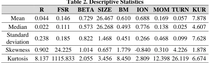
Table 2. Descriptive Statistics

R FSR BETA SIZE BM ION MOM TURN KUR Mean 0.044 0.146 0.729 26.467 0.610 0.688 0.169 0.057 7.878 Median 0.022 0.111 0.573 26.268 0.493 0.776 0.138 0.025 4.607 Standard

deviation 0.238 0.185 0.822 1.468 0.451 0.266 0.468 0.099 7.628 Skewness 0.902 24.225 1.014 0.657 1.779 -0.840 0.310 4.226 1.878 Kurtosis 8.137 1115.833 2.055 3.456 8.450 2.809 12.398 26.119 6.674

Notes: R:Quarterly stock return, FSR:Firm-Specific Risk (based on return’s SD), BETA:Systematic risk, SIZE: size, BM:ratio of book value to market value, ION:institutional ownership, MOM:momentum, TURN:turnover, KUR:Kurtosis.

As it is presented in Table (2), the mean of the quarterly stock return in the sample is 4.4% and its SD is 23.8%. The beta mean of the stocks of firms under study were 0.73 and the mean of the ratio of book value to market value is 0.61. Kurtosis of most variables except institutional ownership is over 3 referring positive kurtosis of those variables. The mean of six-month momentum is 16.9%.

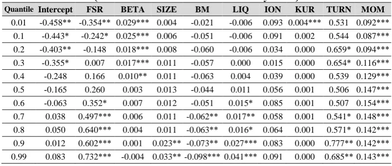
Table 3. The Results of Testing the Relationship between FRS and Return without Industry

(FRS Based on Return’s SD and 15 Day Limit)

Quantile Intercept FSR BETA SIZE BM LIQ ION KUR TURN MOM

0.01 -0.458** -0.354** 0.029*** 0.004 -0.021 -0.006 0.093 0.004*** 0.531 0.092***

0.1 -0.443* -0.242* 0.025*** 0.006 -0.051 -0.006 0.091 0.002 0.544 0.087***

0.2 -0.403** -0.148 0.018*** 0.008 -0.060 -0.006 0.034 0.000 0.659* 0.094***

0.3 -0.355* 0.007 0.017*** 0.011 -0.057 0.000 0.015 0.000 0.654* 0.116***

0.4 -0.248 0.166 0.010** 0.011 -0.063 0.004 0.039 0.000 0.539 0.129***

0.5 -0.165 0.260 0.003 0.013 -0.044 0.011 0.056 0.001 0.506 0.147***

0.6 -0.063 0.352* 0.007 0.012 -0.051 0.015* 0.085 0.001 0.507 0.154***

0.7 0.038 0.497*** 0.006 0.011 -0.062** 0.017** 0.058 0.001 0.541* 0.148***

0.8 0.050 0.640*** 0.004 0.011 -0.063** 0.016* 0.064 0.001 0.571* 0.142***

0.9 0.012 0.602*** 0.001 0.023** -0.073** 0.027*** 0.083 0.000 0.777** 0.142***

0.99 0.083 0.732*** -0.004 0.033** -0.098*** 0.041*** 0.091 0.000 0.685** 0.143***

Notes: FSR:Firm-Specific Risk, BETA:Systematic risk, SIZE:size, BM:ratio of book value to market value, LIQ:liquidity, ION:institutional ownership, MOM: momentum, TURN: turnover, KUR:Kurtosis.

“***”, “**” and “*” indicate statistically significance at level of 99, 95 and 90 percent, respectively.

As it is shown in the table (3), FSR coefficient of the first percentile is -0.354 which is significant at the 95% level of confidence. In the tenth percentile, this coefficient increases to -0.242 and is still significant at the 90% level of confidence. Gradually, by approaching the right side of the distribution, the value of FSR coefficient increases. This increase in 20th to 50th _{percentiles is not statistically significant, and after that, is}

empirical findings on the direction of FSR and stock return as caused by ignoring the effect of skewness of return distribution.

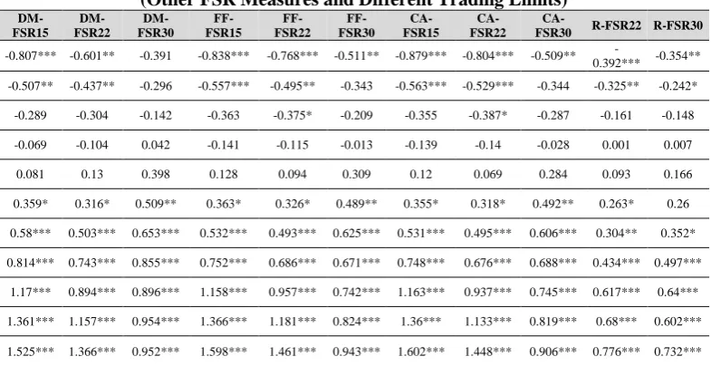
Model (10) is estimated based on the different measures and trading limits and its results are presented in Table (4).

Table 4. FSR Coefficients Resulting from the Estimation of the Relationship between FSR and Return Regardless of Industry

(Other FSR Measures and Different Trading Limits)

DM-FSR15 DM- FSR22

DM- FSR30

FF- FSR15

FF- FSR22

FF- FSR30

CA- FSR15

CA- FSR22

CA-

FSR30 R-FSR22 R-FSR30

-0.807*** -0.601** -0.391 -0.838*** -0.768*** -0.511** -0.879*** -0.804*** -0.509**

-0.392*** -0.354**

-0.507** -0.437** -0.296 -0.557*** -0.495** -0.343 -0.563*** -0.529*** -0.344 -0.325** -0.242*

-0.289 -0.304 -0.142 -0.363 -0.375* -0.209 -0.355 -0.387* -0.287 -0.161 -0.148

-0.069 -0.104 0.042 -0.141 -0.115 -0.013 -0.139 -0.14 -0.028 0.001 0.007

0.081 0.13 0.398 0.128 0.094 0.309 0.12 0.069 0.284 0.093 0.166

0.359* 0.316* 0.509** 0.363* 0.326* 0.489** 0.355* 0.318* 0.492** 0.263* 0.26

0.58*** 0.503*** 0.653*** 0.532*** 0.493*** 0.625*** 0.531*** 0.495*** 0.606*** 0.304** 0.352*

0.814*** 0.743*** 0.855*** 0.752*** 0.686*** 0.671*** 0.748*** 0.676*** 0.688*** 0.434*** 0.497***

1.17*** 0.894*** 0.896*** 1.158*** 0.957*** 0.742*** 1.163*** 0.937*** 0.745*** 0.617*** 0.64***

1.361*** 1.157*** 0.954*** 1.366*** 1.181*** 0.824*** 1.36*** 1.133*** 0.819*** 0.68*** 0.602***

1.525*** 1.366*** 0.952*** 1.598*** 1.461*** 0.943*** 1.602*** 1.448*** 0.906*** 0.776*** 0.732***

Notes: DM-FSR:FSR on the basis of modified CAPM, FF-FSR:FSR on the basis of three-factor model, CA-FSR:FSR on the basis of four-factor model, R-FSR:FSR on the basis of return’s SD, and 15, 22, and 30 days of minimum trading limits.

“***”, “**” and “*” indicate statistically significance at level of 99, 95 and 90 percent, respectively.

reverse to direct by increasing quantiles.

In order to more accurately analyze the issue, model (11) which considers industry factor, is estimated and the results of which are presented in table (5).

Table 5. The Results of Testing Relationship between FSR and Return. With Industry (FSR Based on Return’s SD and 15 Day Limit)

Quantile Intercept FSR BETA SIZE BM LIQ ION KUR TURN MOM 0.01 -0.279 -0.282 0.031 0.000 0.078 -0.012 0.201** 0.006** 0.492 0.093***

0.1 -0.342 -0.271 0.029 0.002 0.054 -0.013 0.199** 0.006** 0.506* 0.093*** 0.2 -0.309 -0.162 0.031 -0.001 0.067 -0.014 0.166** 0.005 0.411 0.100*** 0.3 -0.251 0.004 0.024 -0.003 0.068 -0.015 0.153** 0.003 0.535* 0.089*** 0.4 -0.351 0.080 0.028 -0.005 0.089 -0.019* 0.087 0.003 0.522 0.103*** 0.5 -0.463 0.083 0.020 0.009 0.043 -0.008 0.024 0.004 0.671 0.090** 0.6 -0.294 0.322 0.010 0.002 0.009 -0.010 0.019 0.002 0.446 0.091** 0.7 -0.258 0.329 0.011 0.010 -0.042 0.001 0.092 0.002 0.451 0.081* 0.8 -0.180 0.339 0.007 0.009 -0.051 0.003 0.084 0.003 0.601** 0.076 0.9 0.061 0.380 0.011 0.004 -0.052 0.009 0.068 0.003 0.614** 0.087* 0.99 0.043 0.381 0.012 0.007 -0.052 0.012 0.064 0.002 0.610** 0.088

Notes: FSR:Firm-Specific Risk, BETA:Systematic risk, SIZE:size, BM:ratio of book value to market value, LIQ: liquidity, ION:institutional ownership, MOM: momentum, TURN:turnover, KUR:Kurtosis.

“***”, “**” and “*” indicate statistically significance at level of 99, 95 and 90 percent, respectively.

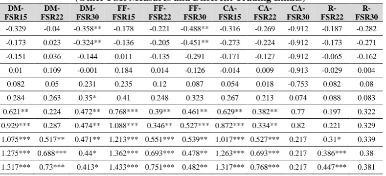
and loses its explanatory power. FSR coefficients resulting from the estimation of model (11) for other measures of FSR and trading limits of 15, 22, and 30 days are presented in table (6).

Table 6. FSR Coefficients Resulting from the Estimation of the Relationship between FSR and Return with the Industry

(Other FSR Measures and Different Trading Limits)

DM-FSR15 DM- FSR22

DM- FSR30

FF- FSR15

FF- FSR22

FF- FSR30

CA- FSR15

CA- FSR22

CA- FSR30

R-FSR22

R-FSR30

-0.329 -0.04 -0.358** -0.178 -0.221 -0.488** -0.316 -0.269 -0.912 -0.187 -0.282

-0.173 0.023 -0.324** -0.136 -0.205 -0.451** -0.273 -0.224 -0.912 -0.173 -0.271

-0.151 0.036 -0.144 0.011 -0.135 -0.291 -0.171 -0.127 -0.912 -0.065 -0.162

0.01 0.109 -0.001 0.184 0.014 -0.126 -0.014 0.009 -0.913 -0.029 0.004

0.082 0.05 0.231 0.235 0.12 0.087 0.054 0.018 -0.753 0.082 0.08

0.284 0.263 0.35* 0.41 0.248 0.323 0.267 0.213 0.074 0.088 0.083

0.621** 0.224 0.472** 0.768*** 0.39** 0.461** 0.629** 0.382** 0.77 0.197 0.322

0.929*** 0.287 0.474** 1.088*** 0.346** 0.527*** 0.872*** 0.334** 0.82 0.221 0.329

1.075*** 0.517** 0.471** 1.213*** 0.551*** 0.539** 1.017*** 0.527*** 0.217 0.31* 0.339

1.275*** 0.688*** 0.44* 1.362*** 0.693*** 0.478** 1.263*** 0.693*** 0.217 0.386*** 0.38

1.317*** 0.73*** 0.413* 1.433*** 0.751*** 0.482** 1.317*** 0.768*** 0.217 0.447*** 0.381

Notes: DM-FSR:FSR on the basis of modified CAPM, FF-FSR:FSR on the basis of three-factor model, CA-FSR:FSR on the basis of four-factor model, R-FSR:FSR on the basis of return’s SD, and 15, 22, and 30 days of minimum trading limits.

“***”, “**” and “*” indicate statistically significance at level of 99, 95 and 90 percent, respectively.

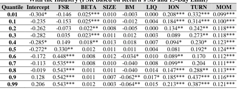
Table 7. Results of Testing the Relationship between FSR and Return: With the Industry (FSR Based on Return’s SD and 15-Day Limit)

Quantile Intercept FSR BETA SIZE BM LIQ ION TURN MOM 0.01 -0.304* -0.146 0.025*** 0.010 -0.003 0.000 0.208*** 0.332*** 0.099***

0.1 -0.235 -0.153 0.025*** 0.010 -0.012 0.004 0.184*** 0.314*** 0.100*** 0.2 -0.262 -0.073 0.022** 0.008 -0.005 0.000 0.134** 0.242** 0.118*** 0.3 -0.282 0.035 0.023*** 0.011 0.012 0.003 0.089 0.273** 0.118*** 0.4 -0.285* 0.149 0.018** 0.013 0.018 0.007 0.094* 0.230* 0.123*** 0.5 -0.272* 0.330** 0.012 0.011 0.011 0.004 0.081 0.192* 0.124*** 0.6 -0.172 0.448*** 0.008 0.012 -0.034* 0.010 0.089** 0.170 0.112*** 0.7 -0.113 0.535*** 0.008 0.010 -0.040 0.008 0.099** 0.204 0.111*** 0.8 -0.019 0.543*** 0.011 0.011 -0.040 0.014 0.147*** 0.288** 0.113*** 0.9 0.128 0.542*** 0.011 0.007 -0.062** 0.017* 0.185*** 0.437*** 0.116*** 0.99 0.206 0.543*** 0.012 0.003 -0.064** 0.015 0.213*** 0.387*** 0.121***

Notes: FSR:Firm-Specific Risk, BETA:Systematic risk, SIZE:size, BM:ratio of book value to market value, LIQ:liquidity, ION:institutional ownership, MOM: momentum, TURN:turnover, KUR:Kurtosis.

“***”, “**” and “*” indicate statistically significance at level of 99, 95 and 90 percent, respectively.

By removing kurtosis in equation (12) the explanatory power of FSR is recovered. Now, FSR coefficient in percentiles 1, 10, and 20 is respectively

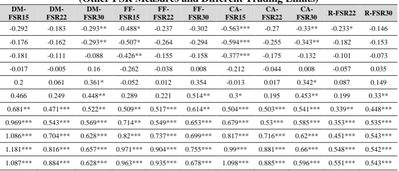
Table 8. FSR Coefficients Resulting From the Relationship between FSR and Return Taking the Industry into Account

(Other FSR Measures and Different Trading Limits)

DM-FSR15

DM- FSR22

DM- FSR30

FF- FSR15

FF- FSR22

FF- FSR30

CA- FSR15

CA- FSR22

CA-

FSR30 R-FSR22 R-FSR30 -0.292 -0.183 -0.293** -0.488* -0.237 -0.302 -0.563*** -0.27 -0.33** -0.233* -0.146

-0.176 -0.162 -0.293** -0.507* -0.264 -0.294 -0.594*** -0.255 -0.343** -0.182 -0.153

-0.181 -0.111 -0.088 -0.426** -0.155 -0.158 -0.377*** -0.175 -0.132 -0.101 -0.073

-0.017 -0.005 0.16 -0.262 -0.038 0.008 -0.212 -0.044 0.008 -0.057 0.035

0.2 0.061 0.361* -0.052 0.012 0.354 -0.013 0.017 0.342* 0.087 0.149

0.466 0.249 0.448** 0.289 0.221 0.514** 0.3* 0.195 0.453** 0.199 0.33**

0.681** 0.471*** 0.522** 0.509** 0.517*** 0.614** 0.504*** 0.503*** 0.541*** 0.339** 0.448***

0.969*** 0.543*** 0.569*** 0.714** 0.549*** 0.653*** 0.679*** 0.53*** 0.585*** 0.353*** 0.535***

1.086*** 0.704*** 0.628*** 0.82*** 0.737*** 0.699*** 0.817*** 0.716*** 0.62*** 0.451*** 0.543***

1.181*** 0.816*** 0.657*** 0.971*** 0.904*** 0.755*** 0.99*** 0.881*** 0.66*** 0.548*** 0.542***

1.087*** 0.884*** 0.628*** 0.963*** 0.935*** 0.678*** 1.098*** 0.885*** 0.596*** 0.551*** 0.543***

Notes: DM-FSR: FSR on the basis of modified CAPM, FF-FSR:FSR on the basis of three-factor model, CA-FSR:FSR on the basis of four-factor model, R-FSR:FSR on the basis of return’s SD, and 15, 22, and 30 days of minimum trading limits.

“***”, “**” and “*” indicate statistically significance at level of 99, 95 and 90 percent, respectively.

As it can be seen, the relationship between FSR and return, regardless of FSR measure and trading limit is always positive and significant in higher quantiles. However, the significance of the relationship in lower quantiles is greatly influences of FSR measure and trading requirement. The results presented in Table (8) reveal that by eliminating kurtosis, industry factor is no longer able to negate FSR’s explanatory power. It must be mentioned that no theoretical basis confirms the reason of the effect of kurtosis on return, but the impact upon stock return has been confirmed in many empirical studies by the fourth moment. On the other hand, the findings presented in table (3) and (4) show that kurtosis regardless of industry is not able to negate the explanatory power of FSR.

5. Conclusion and discussion

cases, and non-significant in some others. Gradually, by increasing percentiles and approaches the right tail of distribution, the relationship between FSR and return becomes positive and statistically significant. The findings of this study confirm the results of Wan & Xiao (2014) on the important role of skewness in the relationship between FSR and return. The findings of this study refer to the effect of industry and kurtosis of return distribution on the relationship between FSR and return. By controlling these two variables, the effect of FSR for FSR measure based on return’s SD is removed. This is not the case if measures based on factor models are used. Economic theories on kurtosis pricing are mostly silent, so that one cannot determine the directing of fourth moment and return changes on the basis of the theoretical background. It might be claimed that this is due to the fact that one cannot specify whether high kurtosis of return distribution is the sign of improvement or deterioration of investment opportunities. In any case, identifying the mutual effect of kurtosis and industry as well as understanding the effect of different FSR measures would help us to better explain the relationship between FSR and return.

Cross-sectional quantile regression analysis confirms that the relationship between FSR and return is affected by the stock return skewness. This finding might explain the contradictory relationship between FSR and return.

References

Ang, A., Hodrick, R J., Xing, Y., & Zhang, X. (2006). The Cross-Section of Volatility and Expected Return. The Journal of Finance, 61, 259-299.

Barnes, M. & Hughes, A. (Tony) W.A. (2002). Quantile regression analysis of the cross section of stock market returns, November. Available at SSRN: http://ssrn.com/abstract=458522.

Bassett Jr, Gilbert W., & Chen, Hsiu-Lang. (2001). Portfolio Style: Return-Based Attribution Using Quantile Regression. Empirical

Economics, 26, 293-305.

Chiang, T C., & Li, J. (2012). Stock returns and risk: Evidence from quantile regression analysis, Journal of Risk and Financial Management, 5, 20-58.

National Bureau of Economic Research, Inc.

Fama, E., & MacBeth, J. (1973). Risk, Return, and Equilibrium: Empirical Tests. Journal of Political Economy, 81, 607-636.

Fatahi, F. & Gerami, A. Qunatile regression. (2004). Paper presented at the 7th Iranian Conference on Statistics, Iran.

Fin, D. E. A. F., Gerrans, P., Singh, A. K. & Powell, R. (2009). Quantile regression: its application in investment analysis. THE FINSIA

JOURNAL OF APPLIED FINANCE, (4), 7-12.

Li, M. L. (2009). Examining the non-monotonic relationship between risk and security returns using the quantile regression approach. Retrieved from http://centerforpbbefr.rutgers.edu/taipeipbfr&d/990515papers/2-1.pdf.

Meligkotsidou, L,. Panopoulou E,. Vrontos, I. D. & Vrontos, S. D. (2012), A Quantile Regression Approach to Equity Premium Prediction. Retrieved from http://ssrn.com/abstract=2061036.

Merton, R. C. (1987). A simple model of capital market equilibrium with incomplete information. Journal of Finance, 42, 483-510.

Morillo, D. (2000). ‘Income mobility with nonparametric quantiles: a comparison of the U.S. and Germany’, Preprint.

Saryal, F. (2009). Rethinking Idiosyncratic Volatility: Is It Really a Puzzel?. Retrieved from www.northernfinance.org/2008/papers /247.pdf