Modeling of CO dispersion from the stack of an Iranian cement Plant
Gholamreza Goudarzi 1, Rajab Rashidi 2,Mohammad Javad Mohammadi 3, Shahram Sadeghi 4, Mehdi Amidnia 5, Yusef Omidi Khaniabadi 6,*
1 Environmental Technologies Research Center (ETRC), Ahvaz Jundishapur University of Medical Sciences, Ahvaz, Iran
2 Department of Occupational Health Engineering, School of Health, Lorestan University of Medical Sciences, Khorramabad, Iran
3 Abadan School of Medical Sciences, Abadan, Iran
4 Environmental Health Research Center, Kurdistan University of Medical Sciences, Sanandaj, Iran 5 Health Center of Andimeshk, Ahvaz Jundishapur University of Medical Sciences, Ahvaz, Iran 6 Health Care System of Karoon, Ahvaz Jundishapur University of Medical Sciences, Ahvaz, Iran
Abstract
The objective of this study was to simulate carbon monoxide (CO) dispersion exited from the stacks of a cement industry in Doroud, Iran by Gaussian Model (GM). Four sampling period was conducted for the measurement of CO from the factory's three-stack flow during a period of one year. The input parameters were the rate of CO emission, meteorological data, factors related to the stack, and factors related to the receptor. Parameters were incorporated in the model and the dispersion of CO during a period of four season was modeled. The southwesterly winds have dominated for the past five years. The highest and the lowest CO levels were estimated at spring and fall seasons with maximum amount of 842.06 and 88.31 µg/m3 within distances of 526 and 960 m away from the cement plant,
respectively. Although the maximum predicted CO concentration at four seasons were lower than the NAAQS standard, the simulation results can be used as a base for reduction of CO emissions rate, because the long-term exposure to emissions of cement plant imposes potentially significant health and environmental impacts.
KEYWORDS: Gaussian Model, Modeling, Carbon monoxide, Cement Plant
Date of submission: 25 Aug 2016, Date of acceptance: 25 Feb 2017
Citation:Goudarzi Gh, Rashidi R, Mohammadi MJ, Sadeghi Sh, Amidnia M, Omidi Khaniabadi Y. Modeling of CO dispersion from the Stack of an Iranian cement industry. J Adv Environ Health Res 2016; 4(4): 199-205
Air pollution due to industrialization is one of the environmental problems globally, especially in developing countries. The increasing development of urban areas, rapid growth of the economy, increase in energy consumption, and population growth are some of the most important factors that threaten health and the environment. 1-5 The major sources of air pollutants are from combined cycle processes, in terms of quality and quantity of fuel combustion. Emissions from fuel combustion that are most important are
CorrespondingAuthors: Yusef Omidi Khaniabadi Email:[email protected]
six-month of the year and is Mazut during the fall and winter period. Therefore, due to the global
concerns regarding CO emissions,
Environmental Protection Agency (EPA) established primary and secondary standards for it in the air. In order to diminish these concerns, it is important to identify how an air pollutant can dispersed in the troposphere.7, 11-14Various parameters such as wind speed and
direction, ground conditions, height of release over ground level, atmospheric stability, etc. have effect on gas dispersion.11, 15, 16There is a
requirement for quantification, identification, and distribution of these pollutants to equation have been used to estimate various pollutants
concentration.18 Application of these
atmospheric models gives useful information for the atmospheric pollution control programs. Gaussian dispersion model combines source linked factors and meteorological parameters to assess pollutant concentration from different sources. The model assumes that the pollutant does not undergo chemical reactions or is not eliminated through other processes including dry or wet deposition. The basic formulation of determining ground level concentration by Gaussian model (GM) in downwind direction
19is presented in Eqs. (1) and (2).
where X is downwind concentration (µg/m3), Q is the emission rate of pollutant
(gr/s), usis wind speed in the stack high (m/s),
δy and δz are standard deviation of lateral and
vertical dispersion (m), zr and zi are the
receptor height above ground level and mixing height (m), respectively. he is also plume
central height (m). Our study was designed to model CO dispersion from the stack of Doroud Cement Plant by GM.
Study area
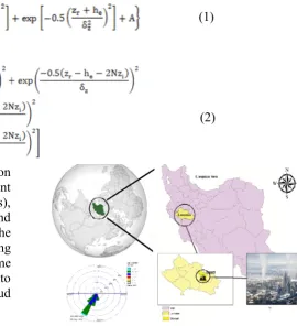
Doroud Cement Plant (33˚29ʹMN, 49˚4ʹME) is one of the productive industries in Doroud City, Lorestan Province, and located in the southwest of Iran (Fig. 1). This factory which manufactures a capacity of 300 tons per day started in 1959. It is located in the vicinity of the residential areas. Several atmospheric contaminants (such as CO) are emitted from appropriate management strategies.17
this industry, which can be harmful for humans that settled downwind the cement factory. Software tools based on Gaussian dispersion manufacture their diminishing facilities with Four sampling period were conducted to
Figure 1. Doroud Cement Plant, the study area CO concentration measuring
measure CO from the factory's three-stack flow in February May, August, and November 2014. In order to measure CO, samples were taken from the stack gas flow based on ASTMD5522-EPACTM-030 standard using Testo (XL350) equipment in a year. To assess the CO atmospheric dispersion in this study area, the GM was used.
Gaussian model
The different steps of estimating CO concentrations in the downwind direction by GM are presented in Equations 3 to 11. For calculation of wind speed in the stack height of cement plant, it is necessary to convert wind
(1)
(6) (3)
(4)
(5)
(7)
(8)
(9) (10) speed at 10 m above ground level as reference
to wind speed in the stack nozzle using Eq. (3). Where u (m/s) and u0(m/s) are the wind speed
in the stack height (Hs, m) and observed wind
speed in reference height (Z0, m), respectively.
Parameter n, the wind profile exponent, is a function of stability category.
The standard theory assumes that a rising buoyant plume entrains ambient air at a rate proportional to both its cross-sectional area and its speed relative to the surrounding air. For the calculation of rising buoyant plume (dh), the parameters of initial velocity of gas flow (w0), the inside stack radius (R0), and
temperature are required. Initial buoyancy flux (Fb) can obtained by Eq. (4):
where Tp0 and Ta0 are the initial plume
temperature and the ambient temperature at stack height, respectively.
For amount of Fb ≥ 55 m4 s-3 in the Pasquill
categories of A-D, buoyant rise was obtained by Eq. (5). In this study, the amount of Fb for classes of A-D was estimated to be lower than 55 m4s-3.
where usis the wind speed at stack height.
In a stable atmosphere, E and F, the final plume rise dh is given by the following equation:
The final effective plume height (H), in meter, is stack height (hs) plus plume rise (dh), which
is presented in Eq. (7) below:
Equations that approximately fit the Pasquill– Gifford curves were used to estimate δy and δz for the rural mode. The equations (8)-(10) were
used to calculate δy and δz.
where TH was computed by Eq. (10).
In Eqs. (8)-(10), the parameter of x is the downwind distance and the coefficients a, b, c and d have been calculated according to the Pasquill stability category.
Meteorological data and stack related factors
For most modeling studies, five years of meteorological data from a representative national weather service station is
recommended. 20 The meteorological data
required for this modeling effort were obtained from surface weather observatory station located close to the cement factory. Five-year results of wind speeds and direction (within the period of 2010-2014) were obtained from meteorological station and then used for drawing of wind rose plot by WRPLOT View Software. For short time periods, a constant representative atmospheric stability was assumed. The surface wind speeds, and wind directions at 10 m above ground level were used in the meteorological analysis to evaluate the environmental impact assessment (HIA) due to CO emissions from the cement factory stack. Moreover, the meteorological data of 2014 were used for drawing of seasonal wind roses.
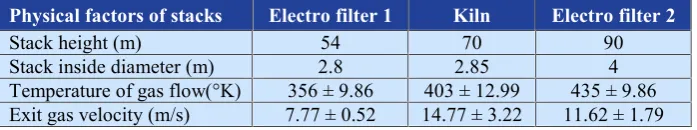
Carbon monoxides samples obtained from three stacks of the cement plant including Electro filter 1 and 2 and Kiln and their averages were applied for the explication of models during a period of four seasons. The temperature of gas flow and exit gas velocity was measured during the sampling period. The stack height, as well as stack inside diameter were used for dispersion modeling of CO as factors related to stack. Table 1 shows the factors related to the three stacks of cement factory.
Table 1. Physical factors related to the three stacks of cement factory Physical factors of stacks Electro filter 1 Kiln Electro filter 2
Stack height (m) 54 70 90
Stack inside diameter (m) 2.8 2.85 4
Fig. 3(a) to (d) shows the seasonal wind rose plots from the daily data recorded by meteorological station. In general, seasonal winds and mountain-valley breezes influences the diurnal climate. The easterly winds were dominant during the spring season and southerly winds were semi-dominant, while with increase in temperature from spring to winter, the wind directions changed from eastern and southern winds toward southeastern. The maximum percentage of time the winds were blown from dominant direction at spring, summer, fall, and winter were 27.5, 17.4, 26.1, and 38.5%, respectively;
which were southerly winds. Seangkiatiyuth et al. (2011) demonstrated that the percentage of time the winds were blown based on the instrument detection limit were 6.9, 17.7, and 47.8%.11
In addition, in warm seasons (spring and summer) especially summer, the changes of wind directions are more than the cold season (fall and winter). Therefore, there were fewer episodes of calm periods in cold season in comparison to the warm season. Abril et al. (2014) reported stronger winds coming from the south direction and these winds were more frequent than the other winds.20Thesefindings
are in line with the results of our study.
Figure 2. Wind rose plots (a) spring, (b) summer, (c) fall, and (d) winter for the study period
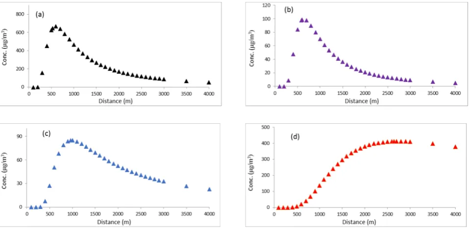
The results of CO dispersion in different distances of emission source at X-axis downwind direction are shown in Fig. 4. As evident in Fig. 4(a) and (b), the maximum predicted concentrations in spring and summer as warm seasons were 688.55 and 98.86 µg/m3,
respectively. Fig. 4 (c) and (d) shows the plots of CO levels at different distance away from the cement plant stacks during fall and winter seasons as cold seasons. As shown, the maximum estimated CO concentrations were 84.98 and 411.88 µg/m3, respectively. The
figures also show that for distances close to the
source, the concentration of pollutants is lower and from these points on to 526, 584, 960, and 2647 m from the source, CO levels rapidly increased in ground level and after drifting downward to a distance of 4000 m, they were found to be 55.52, 5.15, 27.05, and 411.98 μg/m3, respectively. Thus, according to
from the stack of a Jordanian cement plant by AERMOD was 0.086 ppm within 2000 m from
the source. 21 The points of maximum
concentrations calculated by GM are approximately 526, 584, 960, and 2647 m at
downwind direction, respectively. Mohebbi and Baroutian (2006) demonstrated that the point of maximum concentration of pollutant is 750 m downwind of cement plant.17
Figure 3. Dispersion of CO at different distances of cement plant (a) spring, summer, fall, and winter
The worst atmospheric condition was obtained during spring season, where pollution concentrations rapidly increase at ground level. According to the results of our study, maximum CO concentrations were lower than the National Ambient Air Quality Standard (NAAQS) with an average value of 40,000 µg/m3 or 9 ppm. Therefore, this condition has
no health impact on nearby communities in X downwind direction from the south and east of the cement factory. Otaru et al. (2013) reported that due to the fugitive emissions of cement plants, a simulated safety distance of 7,000 m from the source is recommended for human settlement and their activities.22 The highest
and the lowest concentrations of NOX were
predicted in spring and fall seasons, respectively. These findings are in line with the results of a study conducted by Sari et al. (2014). They reported that the prevailing direction of CO was dispersed to the south with the maximum concentration of 60.22 µg/m3at
distance of 750 m from the source. 9
Kahforoshan et al. (2008) showed that the maximum level of CO in selected flare in
Nigeria was 14640 µg/m3, 20 m far from stack
at ground level. 23 Schuhmacher et al. (2004)
indicated that exited pollutants from the cement plant stack were not considered as
causal predictor of mortality, but they have an increase of about 0.2% in risk of asthma attack.
24Momeni et al. (2013) modeled the spread of
air pollution using SCREEN3 and meteorological information. The results of measuring air pollutants using measurement stations indicated that the amount of CO had a lower level than the standards25, this finding is
consistent with the results of the present study.
Although the maximum CO concentrations at four seasons were lower than the NAAQS standard, the simulation results can be used as a base for reduction of CO emissions rate, because the long-term exposure of emissions from cement plant imposes potentially significant health and environmental impacts.
The authors wish to thank the Environmental Group of Doroud Cement Industry.
4. Neisi A, Goudarzi G, Babaei A, Vosoughi M, Hashemzadeh H, Naimabadi A, Mohammadi MJ, Hashemzadeh B. Study of heavy metal levels in indoor dust and their health risk assessment in children of Ahvaz City, Iran. Toxin Rev 2016; 35:16–23
11.Seangkiatiyuth K, Surapipith V, Tantrakarnapa K, Lothongkum AW. Application of the AERMOD modeling system for environmental impact assessment of NO2 emissions from a cement complex. Journal of Environmental Sciences. 2011;23(6):931–40.
2016;3(2):91-7.
15.Dimovska B, Šajn R, Stafilov T, Bačeva K, Tănăselia C. Determination of atmospheric pollution around the thermoelectric power plant using a moss biomonitoring. Air Qual Atmos Health 2014;7:541-57.
17.Mohebbi A, Baroutian S. A Detailed Investigation of Particulate Dispersion from Kerman Cement Plant. Iranian Journal of Chemical Engineering. 2006;3(3):65-74. Hopke PK, Sicard P, De Marco A, et al.
2. Goudarzi G, Daryanoosh SM, Godini H,
20.Abril GA, Wannaz ED, Mateos AC, Pignata ML. Biomonitoring of airborne particulate matter emitted from a cement plant and comparison with dispersion modelling results.
Atmospheric Environment 2014;82: 154-63.
Health risk assessment of exposure to the
5. Khaniabadi Y, Goudarzi G, Daryanoosh S, Borgini A, Tittarelli A, De Marco A. Exposure to PM10,NO2, and O3and impacts on human
health. Environ Sci Pollut Res 2017;
24(3):2781–2789.
10.Khaniabadi YO, Daryanoosh SM, Amrane A, Polosa R, Hopke PK, Goudarzi G, et al. Impact of Middle Eastern Dust storms on human health. Atmospheric Pollution Research 2017; 8(4):606–613.
12.Guttikunda SK, Begum BA, Wadud Z. Particulate pollution from brick kiln clusters in the Greater Dhaka region, Bangladesh. Air Qual
Atmos Health 2013; 6(2):357–36.
Daryanoosh S, Jourvand M, Basiri H. Cardiopulmonary mortality and COPD attributed to ambient ozone. Environmental
Research2017;152:336-41.
16.Khaefi M, Geravandi S, Hassani G, Yari AR,
Soltani F, Dobaradaran S, et al. Association of Particulate Matter Impact on Prevalence of Chronic Obstructive Pulmonary Disease in Ahvaz, Southwest Iran during 2009–2013.
Aerosol and Air Quality Research 2017;
17(1): 230–237.
18.Hess G. Simulation of Photochemical Smog in the Melbourne Air shed: Worst Case Studies. Atmospheric Environment 1989;23:661-9. 19.Mohebbi A, Baroutian S. Numerical Modeling
of Particulate Matter Dispersion from Kerman Cement Plant, Iran. Environ Monit Assess 2007;130:73–82.
21.Abu-Allaban M, Abu-Qudais H. Impact Assessment of Ambient Air Quality by Cement Industry: A Case Study inJordan. Aerosol and
Air Quality Research 2011;11:802-810.
shiftstudy. BMC Pulm Med 2010; 10(19): 1-8.
7. Al Smadi M, Al-Zboon K, Shatnawi K. Assessment of Air Pollutants Emissions from a Cement Plant: A Case Study in Jordan. Jordan of Civil Engineering 2009;3(3):265-82.
6. Goyal P. Present scenario of air quality in Delhi: a case study of CNG implementation. Atmospher Environ 2003;37(38):5423-31.
9. Sari N, Tarumum S, Saryono. Pollutant dispersion modelling (Dust, CO, NOx, and SOx) from palm oil mill stack. Indonesian Journal of Environmental Science and Technology 2014;1(1):28-34.
8. Zeleke Z, Moen B, Bratveit M. Cement dust
exposure and acute lung function: a cross
Daryanoosh SM. Health impact assessment of short-term exposure to NO2 in Kermanshah, Iran using AirQ model. Environmental Health
1. Mohammadi MJ, Goudarzi G, Geravandi S, 13.Khaniabadi YO, Hopke P, Goudarzi G
Yari AR, Ghalani B, Shirali S, et al. Dispersion Modeling of Nitrogen Dioxide in Ambient Air of Ahvaz City. Health Scope.
2016; 5(2): e32540. ,
14.Omidi Y, Goudarzi G, Heidari AM,
megacity of Kermanshah. Public Health Middle -Eastern Dust storms in Iranian Engineering and Management Journal 2017;148:109-116.
3. Nourmoradi H, Khaniabadi YO, Goudarzi G, Daryanoosh SM, Khoshgoftar M, Omidi F, et al. Air Quality and Health Risks Associated With Exposure to Particulate Matter: A Cross-Sectional Study in Khorramabad, Iran. Health
24.Schuhmacher M, Domingo JL, Garreta J. Pollutants emitted by a cement plant: health risks for the population living in the
neighborhood. Environmental Research
2004;95 198-206.
25.Momeni S, Sekhavatjo M. Modeling of air
pollution (Case study: Lavan Island). Sixteenth National Conference on Environmental Health; Tabriz university of medical sciences 2013. https://en.symposia.ir/NCEH16.html. 23.Kahforoshan D, Fatehifar E, Babalou A,
Ebrahimin A, Elkamel A,
Soltanmohammadzadeh J. Modeling and Evaluation of Air pollution from a Gaseous Flare in an Oil and Gas Processing Area. WSEAS Conferences Santander, Cantabria, Spain2008: 23-5.