Vol. 7, No. 1, 2015 Article ID IJIM-00583, 11 pages Research Article
The effects of MHD flow of third grade fluid by means of meshless
local radial point interpolation (MLRPI)
S. Abbasbandy ∗†, E. Shivanian ‡
————————————————————————————————–
Abstract
The meshless local radial point interpolation (MLRPI) method is applied to examine the magneto-hydrodynamic (MHD) flow of third grade fluid in a porous medium. The fluid saturates the porous space between the two boundaries. Several limiting cases of fundamental flows can be obtained as the special cases of present analysis. The variations of pertinent parameters are addressed.
Keywords: Porous medium; Magnetohydrodynamic; Non-Newtonian fluid; Local weak formulation; Meshless local radial point interpolation.
—————————————————————————————————–
1
Introduction
T
heral systems, ranging from natural to Man-e flow inside porous space encounters in sev-manufactured technological ones. Examples of porous space include rye bread, lime stone, oil wells, chemical catalysts, underground aquifers, wood etc. The flows of non-Newtonian fluids [1, 2, 3, 4]) are also significant in many engi-neering applications. Recently, the flows of one-dimensional second grade [5]) and Oldroyd-B [6]) fluids are discussed. Mathematical formulation in these articles has been presented employing the modified Darcy’s law and the mathematical prob-lems were linear. However, the one-dimensional flow of third grade fluid even in steady situation constructs nonlinear differential equation. This equation for flow in porous space through Mod-ified Darcy’s law is more nonlinear. Also, the consideration of grade fluid predicts the shear∗Corresponding author. [email protected] †Department of Mathematics, Imam Khomeini Inter-national University, Ghazvin, 34149-16818, Iran.
‡Department of Mathematics, Imam Khomeini Inter-national University, Ghazvin, 34149-16818, Iran.
thinning/shear thickening effects even in steady flows. Thus, the objective of present article is to consider some fundamental flows of third grade fluid in a porous space. The magnetohydrody-namic (MHD) fluid fills the porous space be-tween the two boundaries. The fluid is electrically conducting in the presence of applied magnetic field. Constant pressure gradient is also consid-ered. Hence we investigate the more general dif-ferential system in usual notation satisfying
d2u dy2 + 2β
d dy
(
du dy
)3
− 1
K
[
1 + 2β
(
du dy
)2]
u−M u=C, (1.1)
u(a) =c u(b) =d, (1.2)
where β, M, K, C are the third grade parame-ter, permeability parameparame-ter, magnetic parameter and pressure gradient parameter. Here u is the velocity in the x-direction.
The main shortcoming of mesh-based meth-ods such as the finite element method (FEM),
the finite volume method (FVM) and the bound-ary element method (BEM) is that these numer-ical methods rely on meshes or elements. In the last two decades, in order to overcome the men-tioned difficulties some techniques the so-called meshless methods have been proposed [7]. This method is used to establish system of algebraic equations for the whole domain of the problem without the use of predefined mesh for the do-main discretization so that set of nodes scattered within the domain of the problem as well as sets of nodes on the boundaries of the domain to rep-resent (but not to discretize) the domain of the problem and its boundaries is used. These sets of scattered nodes are usually called field nodes. There are three types of meshless methods: mesh-less methods based on weak forms such as the ele-ment free Galerkin (EFG) method [8,9], meshless methods based on collocation techniques (strong forms) such as the meshless collocation method based on radial basis functions (RBFs) [10, 11] and meshless methods based on the combina-tion of weak forms and collocacombina-tion technique. Due to the ill-conditioning of the resultant lin-ear systems in RBF-collocation method, various approaches are proposed to circumvent this prob-lem, Refs. [12, 13, 14, 15] being among them. The weak forms are used to derive a set of alge-braic equations through a numerical integration process using a set of quadrature domain that may be constructed globally or locally in the do-main of the problem. In the global weak form methods, global background cells are needed for numerical integration in computing the algebraic equations. To avoid the use of global background cells, a so-called local weak form is used to de-velop the meshless local Petrov-Galerkin (MLPG) method [16, 17, 18, 19, 20, 21, 23]. When a lo-cal weak form is used for a field node, the nu-merical integrations are carried out over a local quadrature domain defined for the node, which can also be the local domain where the test (weight) function is defined. The local domain usually has a regular and simple shape for an in-ternal node (such as sphere, rectangular, etc.), and the integration is done numerically within the local domain. Hence the domain and bound-ary integrals in the weak form methods can eas-ily be evaluated over the regularly shaped sub-domains(spheres in 3D or circles in 2D) and their boundaries. In the literature, several
mesh-less weak form methods have been reported such as diffuse element method (DEM) [24], smooth particle hydrodynamic (SPH) [25, 26], the re-producing kernel particle method (RKPM) [27], boundary node method (BNM) [28], partition of unity finite element method (PUFEM) [29], fi-nite sphere method (FSM) [30], boundary point interpolation method (BPIM) [31] and bound-ary radial point interpolation method (BRPIM) [32]. Liu applied the concept of MLPG and de-veloped meshless local radial point interpolation (MLRPI) method [33,34,35]. In this paper, the problem (1.1)-(1.2) will be solved by meshless lo-cal radial point interpolation (MLRPI) method [36]. It is noticed that for plane Couette flow we have C=c= 0; Plug flow corresponds toC = 0; Poiseuille flow when c = d = 0 and generalized Couette flow when c = 0. Graphical results for different parameters are given and examined.
2
The modified radial point
in-terpolation scheme
In the conventional point interpolation method (PIM) there is a main difficulty that inverse of the polynomial moment matrix (it will be de-fined later) does not often exist. This condition could always be possible depending on the loca-tions of the nodes in the support domain and the terms of monomials used in the basis. If an inap-propriate polynomial basis is chosen for a given set of nodes, it may yield in a badly conditioned or even singular moment matrix [7]. In order to avoid the singularity problem in the polynomial point interpolation method (PIM), the radial ba-sis function (RBF)is used to develop the radial point interpolation method (RPIM) for meshless weak form techniques [34,37,38]. The combina-tion of RPIM and polynomial PIM is described as follows: consider a continuous function u(x) defined in a domain Ω, which is represented by a set of field nodes. The u(x) at a point of interest
x is approximated in the form of
u(x) =
n
∑
i= 1
Ri(x)ai + m
∑
j= 1
pj(x)bj
= RT(x)a + PT(x)b, (2.3)
where Ri(x) is a radial basis function (RBF), n
space coordinatex andm is the number of poly-nomial basis functions. Thepj(x) in Eq. (2.3) is,
in general, chosen in a top-down approach from the Pascal triangle, so that the basis is complete to a desired order and a complete basis is usually preferred. For 1-D problems, we use
PT(x) = {1, x, x2, x3, ..., xm} , (2.4)
For 2-D problems, we shall have
PT(x) =PT(x, y)
={1, x, y, xy, x2, y2, . . . , xm, ym}, (2.5)
and etc. When m= 0, only RBFs are used, oth-erwise the RBF is augmented withm polynomial basis functions. Coefficients ai and bj are
un-known which should be determined. There are some types of RBFs, and the characteristics of RBFs have been widely investigated [10, 39,40]. In the current work, we have chosen the thin plate spline (TPS) as radial basis functions in Eq. (2.3). This RBF is defined as follows:
R(x) = r2m ln(r), m = 1, 2,3, ... . (2.6)
Since R(x) in Eq. (2.6) belongs to C2m−1
(all continuous function to the order 2m − 1), so higher-order thin plate splines must be used for higher-order partial differential operators. For the second-order partial differential equation (1.1), m = 2 is used for thin plate splines (i.e., second-order thin plate splines). In the radial basis function Ri(x), the variable is only the
distance between the point of interest x and a node at xi, i.e., r =| x − xi | for 1-D and
r = √(x − xi)2 + (y − yi)2 for 2-D. In order
to determine ai and bj in Eq. (2.3), a support
domain is formed for the point of interest at x, andnfield nodes are included in the support do-main. Coefficients ai and bj in Eq. (2.3) can
be determined by enforcing Eq. (2.3) to be sat-isfied at these n nodes surrounding the point of interest x. This leads to the system of n linear equations, one for each node. The matrix form of these equations can be expressed as
Us = Rna + Pmb, (2.7)
where the vector of function valuesUs is
Us = {u1, u2, u3, ... , un}T , (2.8)
the RBFs moment matrix is
Rn =
R1(r1) R2(r1) ... Rn(r1)
R1(r2) R2(r2) ... Rn(r2)
..
. ... . .. ...
R1(rn) R2(rn) ... Rn(rn)
n×n
,
(2.9) and the polynomial moment matrix is
Pm =
1 x1 ... xm1
1 x2 ... xm2
..
. ... . .. ... 1 xn ... xmn
n×m
. (2.10)
Also, the vector of unknown coefficients for RBFs is
aT = {a1, a2, a3, ... , an} , (2.11)
and the vector of unknown coefficients for poly-nomial is
bT = {b1, b2, b3, ... , bm} . (2.12)
We notify that, in Eq. (2.9), rk in Ri(rk) is
de-fined as
rk =|xk − xi | . (2.13)
We mention that there arem+nvariables in Eq. (2.7). The additional m equations can be added using the followingm constraint conditions:
n
∑
i= 1
pj(xi)ai = PTma = 0, , j = 1,2, ... , m .
(2.14) Combining Eqs. (2.7) and (2.14) yields the fol-lowing system of equations in the matrix form:
˜ Us =
[ Us 0 ] = [
Rn Pm PTm 0
] [
a b
]
= G˜a,
(2.15) where
˜
Us = {u1u2... un0 0...0} ,
˜
aT = {a1a2... anb1... bm} . (2.16)
Because the matrix Rn is symmetric, the matrix
Gwill also be symmetric. Solving Eq. (2.15), we obtain ˜ a = [ a b ]
= G−1U˜s. (2.17)
Eq. (2.3) can be rewritten as
u(x) = RT(x)a + PT(x)b
= {RT(x),PT(x)} [ a
b
]
.
Now using Eq. (2.17), we obtain
u(x) = {RT(x), PT(x)}G−1Us˜
= ˜ΦT(x) ˜Us, (2.19)
where ˜ΦT(x) can be rewritten as ˜
ΦT(x) = {RT(x), PT(x)} G−1
= {ϕ1(x)ϕ2(x)... ϕn(x)ϕn+1(x) ... ϕn+m(x)} . (2.20)
The firstnfunctions of the above vector function are called the RPIM shape functions correspond-ing to the nodal displacements. We show by the vector ˜ΦT(x) so that it is
˜
ΦT(x) = {ϕ1(x)ϕ2(x)... ϕn(x)} , (2.21)
then Eq. (2.19) is converted to the following one:
u(x) = ˜ΦT(x)Us =
n
∑
i=1
ϕi(x)ui. (2.22)
The derivatives of u(x) are easily obtained as
∂u(x)
∂x =
n
∑
i= 1
∂ϕi(x)
∂x ui,
∂2u(x)
∂x2 =
n
∑
i= 1
∂2ϕi(x)
∂x2 ui. (2.23)
Note that R−n1 usually exists for arbitrary scat-tered nodes and therefore the augmented matrix
G is theoretically non-singular [41, 42]. In addi-tion, the order of polynomial used in Eq. (2.3) is relatively low. We add that the RPIM shape functions have the Kronecker delta function prop-erty, that is
ϕi(xj) =
{
1, i = j , j = 1, 2, ... , n ,
0, i ̸= j , j = 1, 2, ... , n .
(2.24) This is be cause the RPIM shape functions are created to pass through nodal values.
3
The meshless local weak form
formulation
Instead of giving the global weak form, the ML-RPI method constructs the weak form over local quadrature cell such as Ωq, which is a small
re-gion taken for each node in the global domain Ω.
The local quadrature cells overlap with each other and cover the whole global domain Ω. The local quadrature cells could be of any geometric shape and size. In one dimensional problems, they are lines (intervals). The local weak form of Eq. (1.1) foryi ∈Ωiq= (yi−rq, yi+rq), can be written as
∫
Ωi q
d2u
dy2ν(y)dy
−
(
1
K +M
) ∫
Ωi q
uν(y)dy=
2β K ∫ Ωi q ˜ u (
du˜
dy
)2
ν(y)dy
−6β
∫
Ωi q
d2u˜
dy2
(
du˜
dy
)2
ν(y)dy
+C
∫
Ωi q
ν(y)dy, (3.25)
where Ωi
q is the local quadrature domain
associ-ated with the point i, and ν(y) is the Heaviside step function
ν(y) =
{
1, y ∈ Ωq,
0, y /∈ Ωq,
(3.26)
as the test function in each local quadrature do-main. Also, ˜u is the latest available approxima-tion ofuto treat the nonlinearity of the problem by a simple predictor-corrector method. Using integration by parts, one has
∫
Ωi q
d2u(y)
dy2 ν(y)dx
=ν(y)du(y)
dy
y=yi+rq
y=yi−rq
−
∫
Ωi q
du(y)
dy
dν(y)
dy dy
= du(y)
dy
y=yi+rq
y=yi−rq
, (3.27)
and using the test function the following local weak equation will be obtained
du(y)
dy
y=yi+rq
y=yi−rq
−
(
1
K +M
) ∫
Ωi q
udy=
4rqβ
K u˜
(
du˜
dy
)2
−12rqβ
d2u˜
dy2
(
du˜
dy
)2
+ 2rqC.
Applying the radial point interpolation method (RPIM) for the unknown functions, the local inte-gral equation (4.29) is transformed in to a system of algebraic equations with used unknown quan-tities, as described in the next section.
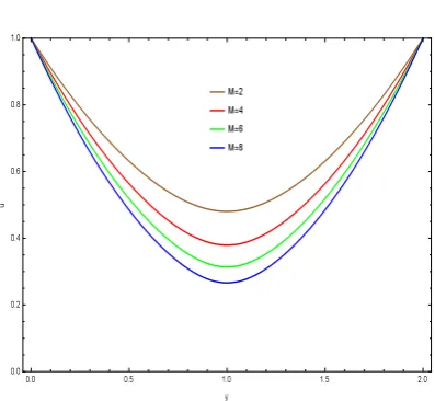
Figure 1: Variation ofM onuwhenK= 1 andβ= 1.
Figure 2: Variation ofKonuwhenM = 1 andβ= 1.
4
Discretization
for
MLRPI
method
In this section, we consider Eq. (4.29) to see how to obtain discrete equations and apply a sim-ple predictor-corrector procedure to overcome the nonlinearity of the problem. Consider N regu-larly located points on the boundary and domain of the problem so that the distance between two consecutive nodes is constant and equal toh. As-suming that u(k)(yi), i = 1,2, ..., N are known,
Figure 3: Variation ofβ onuwhenM = 1 andK= 1.
Figure 4: Variation ofM onuwhenK= 1 andβ = 1.
our aim is to compute u(k+1)(yi), i = 1,2, ..., N. So, we have N unknowns and to compute these unknowns, we need N equations. As it will be described, corresponding to each node we obtain one equation.
Figure 5: Variation ofKonuwhenM = 1 andβ= 1.
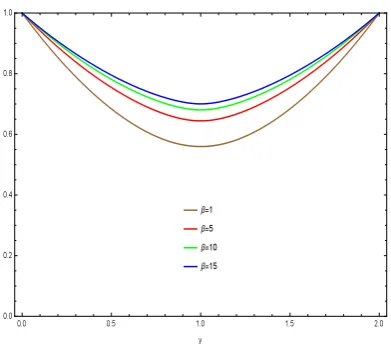
Figure 6: Variation ofβ onuwhenM = 1 andK= 1.
(4.29) yields
N
∑
j=1
u(jk+1)dϕj(y) dy
y=yi+rq
y=yi−rq
−( 1
K +M)
N
∑
j=1
(
∫
Ωi q
ϕj(y)dy)u(jk+1) =
[4rqβ
K (
N
∑
j=1
ϕj(y)u(jk))( N
∑
j=1
dϕj(y)
dy u
(k)
j )2]y=yi
−[12rqβ( N
∑
j=1
d2ϕj(y)
dy2 u (k)
j )( N
∑
j=1
dϕj(y)
dy u
(k)
j )2]y=yi
+ 2rqC, (4.29)
Figure 7: Effect of M on u when C = 1,
K= 1 andβ = 1.
Figure 8: Effect of K on u when C = 1,
M = 1 and β= 1.
or equivalently
N
∑
j=1
[(dϕj(y)
dy
y=yi+rq
−dϕj(y)
dy
y=yi−rq
)
−(1
K +M)(
∫ yi+rq
yi−rq
ϕj(y)dy)]u(jk+1) =
[4rqβ
K (
N
∑
j=1
ϕj(y)u(jk))×
(
N
∑
j=1
dϕj(y)
dy u
(k)
j )2]y=yi
−[12rqβ( N
∑
j=1
d2ϕj(y)
dy2 u (k)
j )×
(
N
∑
j=1
dϕj(y)
dy u
(k)
j )
2]
y=yi
Figure 9: Effect of C on u when β = 1,
M = 1 and K= 1.
Figure 10: Effect of β on u when C = 1,
M = 1 and K= 1.
The number of equations in the above system is
N −2 because we have the number of N −2 in-terior nodes. For nodes which are located on the boundary, from (1.2), we have
uk+1(a) =c, uk+1(b) =d. (4.31)
Therefore, Eqs. (4.30) and (4.31) provide us a linear system of N equations with N unknowns which can be solved iteratively until convergence occurs. In the next section, we have used the cri-teria ∥U(k+1) −U(k)∥∞≤ 10−10 to stop the pro-cedure of solving the system iteratively.
5
Numerical experiments
In this section, we discuss the numerical results for magnetic, porosity and third grade parame-ters.
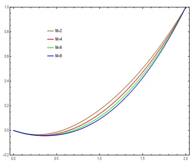
Figure 11: Effect ofM onu whenC = 1,
K= 1 andβ = 1.
Figure 12: Effect ofK onu whenC = 1,
M = 1 and β= 1.
5.1 Plane Couette Flow Problem
We consider the flow between two boundaries in the absence of pressure gradient. The upper boundary is suddenly moved. Here the mathe-matical problem is
d2u dy2 + 2β
d dy
(
du dy
)3
− 1
K
[
1 + 2β
(
du dy
)2]
u−M u= 0, (5.32)
with boundary conditions
u(0) = 0 u(2) = 1. (5.33)
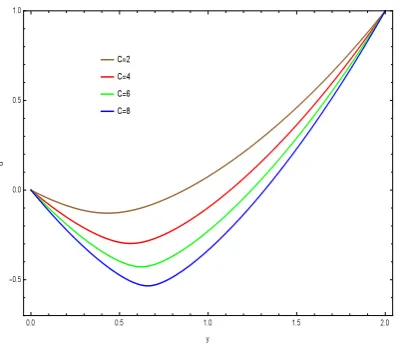
Figure 13: Effect of C on u when β = 1,
M = 1 and K= 1.
Figure 14: Effect of β on u when C = 1,
M = 1 and K= 1.
5.2 Plug Flow Problem
Here we investigate the flow due to sudden motion of two boundaries. The mathematical equation here is
d2u dy2 + 2β
d dy
(
du dy
)3
− 1
K
[
1 + 2β
(
du dy
)2]
u−M u= 0, (5.34)
with boundary conditions
u(0) = 1 u(2) = 1. (5.35)
Figs. 4to6have been displayed for plug flow due to sudden motion of two boundaries.
5.3 Fully developed plane Poiseuille Flow Problem
This subsection deals with the flow in presence of applied pressure gradient. The problem reduces to
d2u dy2 + 2β
d dy
(
du dy
)3
− 1
K
[
1 + 2β
(
du dy
)2]
u−M u=C, (5.36)
with boundary conditions
u(−1) = 0 u(1) = 0. (5.37)
The effects of magnetic, porosity, pressure gra-dient and third grade parameters for fully devel-oped plane Poiseuille flow in the presence of ap-plied pressure gradient are shown in Figs. 7 to
10.
5.4 Generalized plane Couette Flow Problem
Here flow is induced due to applied pressure gra-dient and sudden motion of upper plate. Thus the equation is
d2u dy2 + 2β
d dy
(
du dy
)3
− 1
K
[
1 + 2β
(
du dy
)2]
u−M u=C, (5.38)
with boundary conditions
u(0) = 0 u(2) = 1. (5.39)
Figs. 11 to 14 illustrate the generalized plane Couette flow due to applied pressure gradient and sudden motion of upper plate.
6
Conclusions
In this article, four fundamental flow problems are tested numerically through the employed Scheme. Highly nonlinear problems are solved by this procedure. Through comparative study of the presented results, the following observations are worth-mentioning.
2. Magnitude of velocities in Plug Poiseuille and generalized Couette flows is qualitatively similar to that of Couette flow.
3. Effects of permeability parameter (K) on the velocity in all the considered flows are oppo-site to that of the magnetic parameter.
4. The magnitude of velocity in third grade fluid is much when compared with the vis-cous fluid. This observation holds for all the considered flow cases.
5. Magnitude of velocity in presence of ad-verse pressure gradient is decreased when Poiseuille and generalized Couette flows are studied.
Acknowledgments
The authors acknowledge financial support from the Imam Khomeini International University project IKIU-11552. The authors would like to thank anonymous referees for valuable sugges-tions.
References
[1] M. Nazar, C, Fetecau, D. Vieru, C. Fetecau,
New exact solutions corresponding to the sec-ond problem of Stokes for secsec-ond grade flu-ids, Nonlinear Analysis: Real World Appli-cations 1 (2010) 584-591.
[2] M. Keimanesh, M. M. Rashidi, A. J. Chamkha, R. Jafari, Study of a third grade non-Newtonian fluid flow between two par-allel plates using the multi-step differential transform method, Computers and Math-ematics with Application 62 (2011) 2871-2891.
[3] S. Abbasbandy, T. Hayat, R. Ellahi and S. Asghar, Numerical results of flow in a third grade fluid between two porous walls, Zeitschrift Fur Naturforschung A 64 (2009) 59-64.
[4] S. Abbasbandy, T. Hayat, F. M. Mahomed and R. Ellahi, On comparison of exact and series solutions for thin film flow of a third grade fluid, International Journal of Numer-ical Method in Fluids 61 (2009) 987-994.
[5] W. C. Tan, T. Masuoka, Stokes’ first prob-lem for a second grade fluid in a porous half space with heated boundary, Int. J. Non-Linear Mech. 40 (2005) 512-522.
[6] W. C. Tan and T. Masuoka, Stokes’ first problem for an Oldroyd-B fluid in a porous half space, Phys. Fluids 17 (2005) 23101-23107.
[7] G. Liu,Y. Gu, An introduction to mesh-free methods and their programing, Springer. 2005.
[8] T. Belytschko,Y. Y. Lu, L. Gu,Element-free Galerkin methods, International Journal for Numerical Methods in Engineering 37 (1994) 229-256.
[9] T. Belytschko, Y. Y. Lu, L. Gu,Element free Galerk in methods for static and dynamic fracture, International Journal of Solids and Structures 32 (1995) 2547-2570.
[10] E. Kansa, Multiquadrics – A scattered data approximation scheme with applications to computational fluid-dynamics – I: Surface approximations and partial derivative esti-mates, Computers & Mathematics with Ap-plications 19 (1990) 127-145.
[11] M. Dehghan, A. Shokri,A numerical method for solution of the two dimensional sine-Gordon equation using the radial basis func-tions, Mathematics and Computers inSimu-lation 79 (2008) 700-715.
[12] L. Ling, R. Opfer, R. Schaback, Results on meshless collocation techniques, Engineer-ing Analysis with Boundary Elements 30(4) (2006) 247-253.
[13] L. Ling, R. Schaback, Stable and conver-gent unsymmetric meshless collocation meth-ods, SIAM Journal of Numerical Analysis 46 (2008) 1097-1115.
[15] N. Libre, A. Emdadi, E. Kansa, M. Shekarchi, M. Rahimian, A multi resolution prewavelet-based adaptive refinement scheme for RBF approximations of nearly singular problems, Engineering A nalysis with Bound-ary Elements 33 (2009) 901-914.
[16] S. Atluri, T. Zhu, A new meshless local Petrov-Galerkin (MLPG) approach in com-putational mechanics, Computational Me-chanics 22 (1998) 117-127.
[17] S. Atluri, T. Zhu, A new meshless local Petrov–Galerkin (MLPG) approach to non-linear problems in computer modeling and simulation, Computer Modeling & Simula-tion in Engineering 3 (1998) 187-196.
[18] S. Atluri, T. Zhu, New concepts in meshless methods, International Journal of Numerical Methods in Engineering 13 (2000) 537-56.
[19] S. Atluri, T. Zhu,The meshless local Petrov-Galerkin (MLPG) approach for solving prob-lems in elasto-statics, Computational Me-chanics 25 (2000) 169-179.
[20] M. Dehghan, D. Mirzaei, The meshless lo-cal Petrov–Galerkin (MLPG) method for the generalized two-dimensional non-linear Schr¨odinger equation, Eng. Anal. Bound. Elem. 32 (2008) 747-756.
[21] M. Dehghan, D. Mirzaei, Meshless local Petrov-Galerkin (MLPG) method for the un-steady magnetohydrodynamic (MHD) flow through pipe with arbitrary wall conductivity, Appl. Numer. Math. 59 (2009) 1043-1058.
[22] Y. Gu, G. Liu, A meshless local Petrov-Galerkin (MLPG) method for free and forced vibration analyses for solids, Computational Mechanics 27 (2001) 188-198.
[23] A. Shirzadi, L. Ling, S. Abbasbandy,
Meshlesss imulations of the two-dimensional fractional-time convection-diffusion-reaction equations, Engineering Analysis with Bound-ary Elements 36 (2012) 1522-1527.
[24] B. Nayroles, G. Touzot, P. Villon, General-izing the finite element method: diffuse ap-proximation and diffuse elements, Comput. Mech. 10 (1992) 307-318.
[25] A. G. Bratsos, An improved numerical scheme for the sine-Gordon equation in 2+1 dimensions, Int. J. Numer. Meth. Eng. 75 (2008) 787-799.
[26] P. W.Clear, Modeling conned multi-material heat and mass flows using SPH, Appl. Math. Model. 22 (1998) 981-993.
[27] W. K. Liu, S. Jun, Y. F. Zhang,Reproducing kernel particle methods, Int. J. Numer. Meth. Eng. 20 (1995) 1081-1106.
[28] Y. X. Mukherjee, S. Mukherjee, Boundary node method for potential problems, Int. J. Numer. Meth. Eng. 40 (1997) 797-815. [29] J. M. Melenk, I. Babuska, The partition
of unity finite element method: Basic the-ory and applications, Comput. Meth. Appl. Mech. Eng. 139 (1996) 289-314.
[30] S. De, K. J. Bathe, The method of finite spheres, Comput. Mech. 25 (2000) 329-345. [31] Y. Gu, G. A. Liu, boundary point
interpo-lation method for stress analysis of solids, Computational Mechanics 28 (2002) 47-54. [32] Y. T. Gu, G.R. Liu, A boundary radial
point interpolation method (BRPIM) for 2-D structural analyses, Struct. Eng. Mech. 15 (2003) 535-550.
[33] G. R. Liu, L. Yan, J. G. Wang, Y. T. Gu,
Point interpolation method based on local residual formulation using radial basis func-tions, Struct. Eng. Mech. 14 (2002) 713-732. [34] G. R. Liu, Y. T. Gu, A local radial point interpolation method (LR-PIM) for free vi-bration analyses of 2-D solids, J. Sound Vib. 246 (2001) 29-46.
[35] M. Dehghan, A. Ghesmati, Numerical sim-ulation of two-dimensional sine- gordon solitons via a local weak meshless tech-nique based on the radial point interpolation method (RPIM), Computer Physics Commu-nications, 181 (2010) 772-786.
[37] J. G. Wang, G. R. Liu,A point interpolation meshless method based on radial basis func-tions, Int. J. Numer. Meth. Eng. 54 (2002) 1623-1648.
[38] J. G. Wang, G. R. Liu,On the optimal shape parameters of radial basis functions used for 2-D meshless methods, Comput. Meth. Appl. Math. 191 (2002) 2611- 2630.
[39] C. Franke, R. Schaback, Solving partial dif-ferential equations by collocation using radial basis functions, Applied Mathematics and Computation 93 (1997) 73-82.
[40] M. Sharan, E. J. Kansa, S. Gupta, Appli-cation of the multiquadric method for nu-merical solution of elliptic partial differential equations, Appl. Math. Comput. 84 (1997) 275-302.
[41] M. J. D. Powell, Theory of radial basis function approximation in 1990, in: F.W. Light(Ed.), Adv. Numer. Anal. 4 (1992) 303-322.
[42] H. Wendland, Error estimates for interpo-lation by compactly supported radial basis functions of minimal degree, Journal of Ap-proximation Theory 93 (1998) 258-396.
Saeid Abbasbandy has got PhD de-gree from Kharazmi University in 1996 and now he is the full pro-fessor in Imam Khomeini Interna-tional University, Ghazvin, Iran. He has published more than 200 papers in international journals and conferences. Now, he is working on numerical analysis and fuzzy numerical analysis.
Dr. Elyas Shivanian was born in Zanjan province, Iran in August 26, 1982. He started his mas-ter course in applied mathemat-ics in 2005 at Amirkabir Univer-sity of Technology and has finished MSc. thesis in the field of fuzzy linear programming in 2007. After his Ph.D. in the field of prediction of multiplicity of so-lutions of boundary value problems, at Imam