Vol. 4, No. 4, Year 2012 Article ID IJIM-00191, 9 pages Research Article
Symmetric Error Structure in Stochastic DEA
M. H. Behzadia, M. Mirboloukib∗
(a)Department of Statistics, Science and Research Branch, Islamic Azad University, Tehran, Iran.
(b)Department of Mathematics, Shahre-Rey Branch, Islamic Azad University, Tehran, Iran. ——————————————————————————————————
Abstract
Stochastic programming is an approach for modeling and solving optimization problem that include uncertain data. Chance constrained programming is one of the most impor-tant methods of stochastic programming. In many real world data envelopment analysis (DEA) models, exact amount of data can not be determined. Therefore several researchers proposed methods to evaluate stochastic efficiency of units with random inputs and/or out-puts. Most of these methods are nonlinear. In this paper by introducing symmetric error structure for random variables, a linear from of stochastic CCR is provided. Finally, the proposed model is applied on an example.
Keywords: Data envelopment analysis; Stochastic programming; Symmetric error structure
——————————————————————————————————
1
Introduction
Data Envelopment Analysis (DEA) is a technique based on mathematical programming to assess the efficiency of a set of Decision Making Units (DMUs). Charnes et al. [2] were pioneers in DEA by introducing CCR model. In various fields, many DEA models have been presented to evaluate DMUs with different kinds of data such as deterministic, fuzzy and interval. However, in many practical problems managers deal with units with imprecise data. Thus they need methods to assess their units. In these situations analysts may consider imprecise data as random variables. While working by random variables with considering the possibility for occurrence of unforeseen events, different aspects of the information can be detected. The main advantage of working with random data in DEA is the prediction of efficiencies in future. Given the need to use random data in practical models, Several researchers initiated stochastic DEA models (see [3,4,5,10,11,15]). Subsequently, Li [12], Sengupta [14], Huang and Li [6], Olesen [13], Khodabakhshi [8,9], Behzadi et al.[1] and Jahanshahloo et al. [7] present more stochastic DEA models. Almost
all of these models are nonlinear. In this paper using symmetric error structure for inputs and outputs, deterministic equivalent of CCR model is presented which is a linear model. The paper organized as follows: First the preliminaries on stochastic models and stochastic efficiency is provided in section 2 and then by introducing symmetric error structure the deterministic equivalent of CCR model is obtained in section 3. In section 4 Using numerical example, we will demonstrate how to use the result. Section 5 conclude the paper.
2
Preliminaries
Assume there are n homogeneous DMUs (DM Uj, j = 1, ..., n) such that all the DMUs use m inputs xij (i= 1, ..., m) to produce s outputs yrj (r = 1, ..., s). Also assume that xj = (x1j, ..., xmj) andyj = (y1j, ..., ysj) are nonnegative and nonzero vectors. The set of production possibility set (PPS) is defined as T ={(X, Y)|Y ≥0can be produced by X ≥ 0}. Here we assume thatT =TCCR in which:
TCCR ={(X, Y)| n
∑
j=1
λjXj ≤X, n
∑
j=1
λjYj ≥Y, λj ≥0}.
The input oriented CCR model [2] to estimate the efficiency of DM Uo,o∈ {1, ..., n} is
min θ
s.t. n
∑
j=1
xijλj ≤θxio, i= 1, ..., m,
n
∑
j=1
yrjλj ≥yro, r = 1, ..., s,
λj ≥0, j = 1, ..., n.
(2.1)
In model (2.1) it is assumed that inputs and outputs are deterministic values. Now, let us assume that these data are random variables i.e. ˜Xj = (˜x1j, ...,x˜mj) and ˜Yj = (˜y1j, ...,y˜sj) are random input and output vectors ofDM Uj,j= 1. . . , nandXj = (x1j, ..., xmj)∈Rm+ and Yj = (y1j, ..., ysj) ∈Rs+ stand for corresponding vectors of expected values of input and output for it. All input and output components have been considered to be normally distributed i.e.
˜
xij ∼N(xij, σij2), i= 1, ..., m,
˜
yrj ∼N(yrj, σ
′2
rj), r= 1, ..., s.
Therefore the chance constrained model related to input oriented stochastic CCR model for evaluating DM Uo, o∈ {1, ..., n}is follows:
min θ
s.t. p{ n
∑
j=1
˜
xijλj ≤θx˜io} ≥1−α, i= 1, ..., m,
p{ n
∑
j=1
˜
yrjλj ≥y˜ro} ≥1−α, r= 1, ..., s,
λj ≥0, j= 1, ..., n.
where in the above model, p means “probability” and α is a level of error between 0 and 1, which is a predetermined number. The deterministic equivalent of model (2.2) which is obtained by Cooper et al.[4] is follows:
min θ
s.t. n
∑
j=1
xijλj+s−i −Φ−1(α)vi=θxio, i= 1, ..., m,
n
∑
j=1
yrjλj −s+r + Φ−1(α)ur=yro, r= 1, ..., s,
v2i =∑ j̸=o
∑
k̸=o
λjλkcov(˜xij,x˜ik) + 2(λo−θ)
∑
j̸=o
λjcov(˜xij,x˜io)+
(λo−θ)2var(˜xio), i= 1, ..., m,
u2r =∑ j̸=o
∑
k̸=o
λjλkcov(˜yrj,y˜rk) + 2(λo−1)
∑
j̸=o
λjcov(˜yrj,y˜ro)+
(λo−1)2var(˜yro), r= 1, ..., s, s−i ≥0, s+
r ≥0, i= 1, ..., m, r= 1, ..., s, λj ≥0, ur≥0, vi ≥0 j= 1, ..., n, r= 1, ..., s, i= 1, ..., m.
(2.3)
Here, Φ is the cumulative distribution function of the standard normal distribution and Φ−1(α), is its inverse in level ofα. model (2.3) is an nonlinear and quadratic programming model. Also,DM Uo is defined a stochastic efficient DMU in level ofαif and only ifθ∗ = 1 in the optimal solution of model (2.3).
3
Stochastic Efficiency Based on Symmetric Error
Struc-ture
In this section symmetric error structure for random inputs and outputs is introduced. Then using this structure the stochastic CCR model convert to a deterministic linear model.
Assume related inputs and outputs of DM Uj,j= 1, ..., nare as following structure:
˜
xij =xij +aijε˜ij, i= 1, ..., m, ˜
yrj =yrj +brjξ˜rj, r= 1, ..., s.
(3.1)
whereaij andbrj are nonnegative real values. Also, ˜εij and ˜ξrj are random variables with normal distributions, ˜εij ∼N(0,σ¯2) and ˜ξrj ∼N(0,σ¯2). Therefore ˜εij and ˜ξrj are errors of inputs and outputs in contrast to the mean values respectively. Since normal distribution is symmetric then the structure in expression (3.1) is named symmetric error structure. Also, the following relations are resulted from expression (3.1):
˜
xij ∼N(xij,σ¯2a2ij), ˜
yrj ∼N(yrj,σ¯2b2rj).
Similarly assumerth output of every DMUs are uncorrelated, too. i.e. for everyj ̸=k,
Cov(˜εij,ε˜ik) = 0, i= 1, ..., m, Cov( ˜ξrj,ξ˜rk) = 0, r= 1, ..., s.
(3.2)
Therefore according to relations (3.1) and (3.2), it can be considered a same error for all DMUs, i.e. ˜εi = ˜εij and ˜ξr = ˜ξrj, for everyj= 1, ..., n,i= 1, ..., mand r= 1, ..., s.
Now, consider ith input constraint of model (2.2),
p{ n
∑
j=1
˜
xijλj ≤θx˜io} ≥1−α (3.3)
Let ˜hi = n
∑
j=1
λjx˜ij −θx˜io. So (3.1) and (3.2) result:
˜ hi= (
n
∑
j=1
λjxij −θxio)+˜εi( n
∑
j=1
λjaij−θaio)
Therefore,
˜ hi∼N
(
n
∑
j=1
λjxij−θxio),σ¯2( n
∑
j=1
λjaij −θaio)
2
From the above expression and normal distribution properties, the stochastic constraint (3.3) can be converted to the following deterministic equivalent:
n
∑
j=1
λjxij −Φ−1(α)¯σ
n ∑ j=1
λjaij −θaio
≤θxio. (3.4)
Similarly, rth output constraint of model (2.2) can be converted to
n
∑
j=1
λjyrj+ Φ−1(α)¯σ
n ∑ j=1
λjbrj−bro
≥yro (3.5)
Therefore from (3.4) and (3.5), deterministic equivalent of model (2.2) is
min θ
s.t. n
∑
j=1
λjxij−Φ−1(α)¯σ
n ∑ j=1
λjaij−θaio
≤θxio,i= 1, ..., m, n
∑
j=1
λjyrj + Φ−1(α)¯σ
n ∑ j=1
λjbrj −bro
≥yro, r= 1, ..., s, λj ≥0, j = 1, ..., n.
Model (3.6) is a nonlinear programming but it can be converted to linear using the following transformations:
n
∑
j=1
λjaij −θaio
= (p+i +p−i ), i= 1, ..., m, n
∑
j=1
λjaij−θaio= (p+i −p−i ), i= 1, ..., m,
p+i p−i = 0, i= 1, ..., m,
n
∑
j=1
λjbrj−bro
= (qr++q−r), r= 1, ..., s, n
∑
j=1
λjbrj −bro= (qr+−qr−), r= 1, ..., s,
q+rqr−= 0, r= 1, ..., s,
p+i ≥0, p−i ≥0, q+r ≥0, q−r ≥0.
By substituting the above relation in model (3.6), we have:
min θ
s.t. n
∑
j=1
λjxij−Φ−1(α)¯σ(p+i +p−i )≤θxio,i= 1, ..., m, n
∑
j=1
λjyrj+ Φ−1(α)¯σ(qr++qr−)≥yro, r= 1, ..., s, n
∑
j=1
λjaij−θaio=p+i −p−i ,i= 1, ..., m, n
∑
j=1
λjbrj −bro=qr+−q−r, r= 1, ..., s,
p+i p−i = 0, i= 1, ..., m, qr+q−r = 0, r= 1, ..., s,
λj, p+i , p−i , qr+, qr−≥0, j = 1, ..., n, i= 1, ..., m, r= 1, ..., s.
(3.7)
Model (3.7) is nonlinear because of the existence of constraints p+i p−i = 0 and qr+qr− = 0. It must be noted that for every linear problem which has an optimal solution, there is at least a basic optimal solution. Model (3.7) without constraints p+i p−i = 0 and qr+qr− = 0 is a linear model while in every its optimal basic solutions at least one of p+i and p−i for every i = 1, ..., mand at least one of qr+ and q−r for every r = 1, ..., s is zero. Therefore constraints p+i p−i = 0 and q+rqr− = 0 will be satisfied in optimal basic solutions of linear model. Thus, assuming the use of optimal basic solution detector algorithms (for example
equivalent of model (2.2) is
θ∗(α) = min θ
s.t.
n
∑
j=1
λjxij −Φ−1(α)¯σ(p+i +p−i )≤θxio,i= 1, ..., m, n
∑
j=1
λjyrj + Φ−1(α)¯σ(q+r +qr−)≥yro, r= 1, ..., s, n
∑
j=1
λjaij −θaio =p+i −p−i ,i= 1, ..., m, n
∑
j=1
λjbrj−bro =qr+−qr−, r= 1, ..., s,
λj, p+i , p−i , q+r, q−r ≥0, j= 1, ..., n, i= 1, ..., m, r= 1, ..., s.
(3.8)
Theorem 3.1. 0< θ∗(α)≤1 for every α <0.5 in model (3.8).
Proof. Let θ= 1, λo = 1, λj = 0; j ̸= o, pi+ = 0, p−i = 0; i = 1, ..., m, qr+ = 0, q−r = 0; r = 1, ..., s. This solution is feasible for model (3.8) in every α levels of error. Since this model is minimizing then θ∗(α)≤1. If α < 0.5, then Φ−1(α) <0. Therefore inputs and output constraint of model (3.8) results
n
∑
j=1
λ∗jxij ≤θ∗xio, i= 1, ..., m,
n
∑
j=1
λjyrj ≥yro,r= 1, ..., s.
Now supposeθ∗(α)≤0 (by contradiction hypothesis). Sincexij ≥0,xj ̸= 0 andλ∗j ≥0 by definition then the first and the last of above inequalities results λ∗j = 0; j = 1, ..., n and yrj ≤0 respectively. which is a contradiction by definitions yrj ≥0, r = 1, ..., s and yj ̸= 0. Thus θ∗(α)≥0.
Theorem 3.2. θ∗(α′)≤θ∗(α) for everyα≤α′ in model (3.8).
Proof. Let (θ∗,λ∗, p+∗, p−∗, q+∗, q−∗) be an optimal solution of model (3.8) in α level of error. Since Φ−1(α) is nondecreasing function, so Φ−1(α)≤Φ−1(α′) and
0≥ n
∑
j=1
λ∗jxij−Φ−1(α)¯σ(p+i∗+p−∗i )−θ∗xio≥ n
∑
j=1
λ∗jxij −Φ−1(α′)¯σ(p+i ∗+p−∗i )−θ∗xio,
0≤ n
∑
j=1
λ∗jyrj+ Φ−1(α)¯σ(qr+∗+qr−∗)−yro≤ n
∑
j=1
λ∗jyrj+ Φ−1(α′)¯σ(qr+∗+qr−∗)−yro.
Corollary 3.1. Theorem 3.1 shows ifDM Uo is efficient inα′ level of error, then it would
be efficient for everyα < α′. Also, ifDM Uois inefficient inα′ level of error, then it would
be inefficient for every α′ < α. It is noteworthy to say that for 0.5 level of error model (3.8) is CCR model with mean of data. Thus if a DMU is efficient in CCR mean model, then it would be efficient for every α < 0.5. It means permanent efficient DMUs can be detected by assessing them in α = 0.5. Also, if a DMU is inefficient in α = 0, then it remain inefficient in all levels of error. Since Φ−1(0) =−∞ but Φ−1(0,001)≃ −3, so by assessing DMUs in α= 0,001 almost all permanent inefficient DMUs can be detected.
4
An application
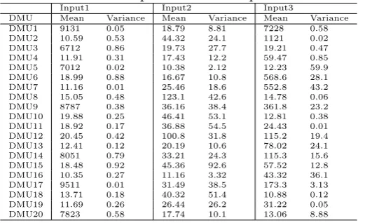
In this section, we consider 20 branches of an Iranian bank with three stochastic inputs and five stochastic outputs which are mentioned in Table 4.1.
Table 4.1. inputs and outputs
input 1 personal rate (weighted combination of personal qualifications, quantity, education and others) input 2 payable benefits (of all deposits)
input 3 delayed requisitions (delay in returning ceded loans and other facilities)
output 1 facilities (sum of business and individual loans)
output 2 amount of deposits (of current, short duration and long duration accounts) output 3 received benefits (of all ceded loans and facilities)
output 4 received commission (on banking operations, issuance guaranty, transferring money and others) output 5 other resources of deposits
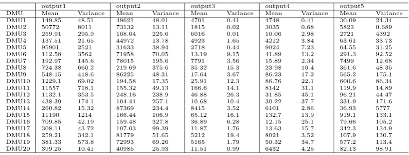
These data based on consideration ten successive months have normal distribution and their scaled parameters are presented in Tables 4.2 and 4.3. We want to assess the total performance of these units. We suppose that ¯σ = 1 in symmetric error structure, thus aij =
√
V ar(˜xij) andbrj =
√
V ar(˜yrj). Here by running model (3.8) stochastic efficien-cies of all branches are evaluated and results are gathered in Table 4.4.
Table 4.2 Estimated parameters of inputs normal distributions.
Input1 Input2 Input3
DMU Mean Variance Mean Variance Mean Variance
DMU1 9131 0.05 18.79 8.81 7228 0.58
DMU2 10.59 0.53 44.32 24.1 1121 0.02
DMU3 6712 0.86 19.73 27.7 19.21 0.47
DMU4 11.91 0.31 17.43 12.2 59.47 0.85
DMU5 7012 0.02 10.38 2.12 12.23 59.9
DMU6 18.99 0.88 16.67 10.8 568.6 28.1
DMU7 11.16 0.01 25.46 18.6 552.8 43.2
DMU8 15.05 0.48 123.1 42.6 14.78 0.06
DMU9 8787 0.38 36.16 38.4 361.8 23.2
DMU10 19.88 0.25 46.41 53.1 12.81 0.38
DMU11 18.92 0.17 36.88 54.5 24.43 0.01
DMU12 20.45 0.42 100.8 31.8 115.2 19.4
DMU13 12.41 0.12 20.19 10.6 78.02 24.1
DMU14 8051 0.79 33.21 24.3 115.3 15.6
DMU15 18.48 0.92 45.36 92.6 57.52 12.8
DMU16 10.35 0.27 11.16 3.32 43.32 36.1
DMU17 9511 0.01 31.49 38.5 173.3 3.13
DMU18 13.71 0.18 40.32 51.4 10.88 0.12
DMU19 11.69 0.26 26.44 26.2 31.22 0.05
output1 output2 output3 output4 output5
DMU Mean Variance Mean Variance Mean Variance Mean Variance Mean Variance
DMU1 149.85 48.51 49621 48.01 4701 0.41 4748 0.41 30.09 24.34
DMU2 50772 8011 73132 13.11 1815 0.02 3035 0.68 5823 0.689
DMU3 259.91 295.9 108.04 225.6 6016 0.01 10.06 2.98 2721 4392
DMU4 137.51 21.65 44972 13.78 4923 1.65 4212 3.84 63.61 33.73
DMU5 95901 2521 31633 38.94 2718 0.44 9024 7.23 64.55 31.25
DMU6 112.58 3562 71958 70.05 13.19 9.15 41.89 13.2 291.3 92.52
DMU7 192.97 145.6 78015 195.6 7791 3.56 15.89 2.34 7499 12.68
DMU8 724.38 660.2 219.69 375.6 35.32 15.3 23.98 10.4 361.6 48.35
DMU9 548.15 418.6 86225 48.31 17.64 3.67 86.23 17.2 565.2 175.1
DMU10 1229.1 69.02 194.58 17.35 25.91 12.3 86.76 22.1 600.6 86.34
DMU11 11557 718.1 155.32 49.13 166.6 14.1 8142 31.1 119.9 14.89
DMU12 1132.1 353.5 248.16 238.9 46.88 26.3 31.85 45.1 96.21 44.47
DMU13 438.39 174.1 104.41 257.1 10.68 10.4 30.22 37.7 331.9 171.6
DMU14 260.82 15.32 87369 234.4 8415 3.52 6101 2.86 36.93 5777
DMU15 11190 1214 166.44 106.9 65.12 16.1 132.7 13.9 919.1 133.1
DMU16 709.85 42.19 159.48 327.8 36.89 6.28 12.15 25.1 79.66 105.2
DMU17 308.11 43.72 107.03 99.39 11.87 1.76 13.63 15.7 342.3 134.9
DMU18 259.21 342.1 81779 51.65 5212 19.4 8021 3.52 107.9 130.7
DMU19 381.33 573.8 72993 69.26 5165 1.79 50.32 34.7 577.2 113.4
DMU20 399.25 10.41 40985 25.93 11.51 0.99 6432 4.25 82.13 98.91
Table 4.4 Computational results of model (3.8).
DMU α= 0.999 α= 0.5 α= 0.1 α= 0.05 α= 0.001
DMU1 0.03 0.59 0.67 0.7 0.77
DMU2 0 1 1 1 1
DMU3 0.02 1 1 1 1
DMU4 0.1 0.28 0.3 0.3 0.34
DMU5 -1.81 0.49 0.98 1 1
DMU6 0.03 0.92 0.97 0.99 1
DMU7 0.02 0.48 0.56 0.58 0.66
DMU8 0.12 1 1 1 1
DMU9 0.08 1 1 1 1
DMU10 0.51 1 1 1 1
DMU11 1 1 1 1 1
DMU12 0.1 0.79 0.89 0.91 0.99
DMU13 1 0.91 0.95 0.96 0.99
DMU14 0.01 0.69 0.73 0.74 0.77
DMU15 1 1 1 1 1
DMU16 0.06 1 1 1 1
DMU17 0.08 0.93 0.99 1 1
DMU18 0.08 0.56 0.61 0.62 0.67
DMU19 0.16 1 1 1 1
DMU20 0.04 0.46 0.54 0.57 0.73
Results in Table 4.4 show the efficiency may be negative while the level of error is less than half (note efficiency of DM U5 in 0.999 level of error). Also, efficiency of each DMU
increases during decreasing level of error. DMUs 2, 3, 8, 9, 10, 11, 15, 16 and 19, which are efficient in 0.5 level of error, are permanent efficient DMUs. DMUs 1, 4, 7, 12, 13, 14, 18 and 20, which are inefficient in 0.001 level of error, are permanent inefficient DMUs.
5
Conclusion
References
[1] MH. Behzadi, N. Nematollahi, M. Mirbolouki, Ranking Efficient DMUs with Stochas-tic Data by Considering Inecient Frontier, International Journal of Industrial Math-ematics 1 (2009) 219-226.
[2] A. Charnes, WW. Cooper, E. Rhodes, Measuring the efficiency of decision making units, European Journal of Operational Research 2 (1978) 429-444.
[3] WW. Cooper, H. Deng, Z. Huang, SX. Li, Chance constrained programming ap-proaches to congestion in stochastic data envelopment analysis, European Journal of Operational Research 155 (2004) 487-501.
[4] WW. Cooper, Z. Huang, S. Li,Satisficing DEA models under chance constraints, The Annals of Operations Research 66 (1996) 259-279.
[5] WW. Cooper, RG. Thompson, RM. Thrall, Introduction: Extensions and new devel-opments in DEA, Annals of Operations Research 66 (1996) 3-46.
[6] Z. Huang, SX. Li, Stochastic DEA models with different types of input-output distur-bances, Journal of Productivity Analysis 15 (2001) 95-113.
[7] GR. Jahanshahloo, MH. Behzadi, M. Mirbolouki,Ranking Stochastic Efficient DMUs based on Reliability, International Journal of Industrial Mathematics 2 (2010) 263-270.
[8] M. Khodabakhshi,Estimating most productive scale size with stochastic data in data envelopment analysis, Economic Modelling 26 (2009) 968-973.
[9] M. Khodabakhshi, M. Asgharian,An input relaxation measure of efficiency in stochas-tic data envelopment analysis, Applied Mathematical Modelling 33 (2008) 2010-2023.
[10] KC. Land, CAK. Lovell, S. Thore, Productive efficiency under capitalism and state socialism: The chance constrained rogramming approach, Public Finance in a World of Transition 47 (1992) 109-121.
[11] KC. Land, CAK. Lovell, S. Thore,Productive efficiency under capitalism and state socialism: An empirical inquiry using chanceconstrained data envelopment analysis, Technological Forecasting and Social Change 46 (1994) 139-152.
[12] SX. Li, Stochastic models and variable returns to scales in data envelopment analysis, European Journal of Operational Research 104 (1998) 532-548.
[13] OB. Olesen, Comparing and Combining Two Approaches for Chance Constrained DEA, Discussion paper, The University of Southern Denmark, (2002).
[14] JK. Sengupta, Efficiency analysis by stochastic data envelopment analysis, Applied Economics Letters 7 (2002) 379-383.