ISSN: 2374-2348 (Print), 2374-2356 (Online) Copyright © The Author(s).All Rights Reserved. Published by American Research Institute for Policy Development DOI: 10.15640/arms.v7n2a4 URL: https://doi.org/10.15640/arms.v7n2a4
An
𝐅 −
Type Multiple Testing Approach for Assessing Randomness of Linear Mixed
Models
Marco Barnabani
1Abstract
In linear mixed models the assessing of the significance of all or a subset of the random effects is often of primary interest. Many techniques have been proposed for this purpose but none of them is completely satisfactory. One of the oldest methods for testing randomness is the F −test but it is often overlooked in modern applications due to poor statistical power and non-applicability in some important situations. In this work a two-step procedure is developed for generalizing an F −test and improving its statistical power. In the first step, by comparing two covariance matrices of a least squares statistic, we obtain a ”repeatable” F −type test. In the second step, by changing the projected matrix which defines the least squares statistic we apply the test repeteadly to the same data in order to have a set of correlated statistics analyzed within a multiple testing approach. The resulting test is sufficiently general, easy to compute, with an exact distribution under the null and alternative hypothesis and, perhaps more importantly, with a strong increase of statistical power with respect to the F −test.
keywords: Linear Mixed Models; Hypothesis testing; Comparison of matrices; F-distribution; Beta binomial distribution.
1 Introduction
In longitudinal studies with subjects measured repeatedly across time there has been increasingly more attention on linear mixed-effects models (Laird and Ware, 1982) because they can incorporate within-cluster and between-cluster variations. Linear mixed effect models (LME models) can be viewed as an extension of linear regression models (LR
models) where one or more subject-specific latent variables are included to account for within-subject dependency. Typically, an additional random effect is included for each regression coefficient which is expected to vary among subjects and it becomes important to assess the randomness of all or a subset of parameters. A linear mixed model can be regarded as a two-stage model (Laird, 2004) where in the first stage it may be viewed as a set of standard regression models with the matrix of covariates and the random effects design matrix ”merged” in a unique matrix and the parameter vector which includes both fixed and random parameters or the sum of both (Rocha and Singer, 2017). In the second stage a specification of the mean and the variance of the random effects are assumed.When faced with this representation, we can ask whether the ”enlarged” parameters vector is fixed, random or has both fixed and random elements. In order to address the issue of which model is more suitable, one might use standard model selection measures based on information criteria such as the widely used Akaike Information Criteria (AIC; Akaike(1973)), the Bayesian Information Criteria (BIC; Schwarz(1978)) or the conditional Akaike Information Criterion (cAIC, Vaida and Blanchard(2005)). We refer to the paper of Muller etal.(2013) for a review of these approaches and other methods such as shrinkage methods like the LASSO (Tibshirani, 1996), Fence methods (Jiang etal., 2008) and Bayesian methods. The validity of all the methods proposed depends on the underlying assumptions.
The review paper of Muller etal.(2013) gives an overview of the limits and most important findings of above-mentioned approaches, extracting information from some published simulation results.
As is known, one of the major drawbacks of these approaches is that they fail to give any measure of the degree of uncertainty of the model chosen. The value they produce does not mean anything by itself.Alternatively, because model selection is closely related to hypothesis testing, the choice between an LR model and an LME model and the evaluation of its uncertainty could be conducted by assessing the significance of all or a subset of the random effects. This normally involves the use of hypothesis tests to detect whether one or more variance components are equal to zero. Extensive research has been conducted into testing the significance of random effects in linear mixed models. Arguably, the main challenge has been how to deal with the fact that under the null hypothesis, the variance lies on the boundary of the parameter space, meaning that the likelihood ratio as well as the score and Wald tests are not asymptotically chi-squared distributed. Consequently, in large samples they lead to a power lower than that of the standard case and in finite samples they tend to produce conservative tests.Over the past two decades, these difficulties in conservatism and the somewhat strict model assumptions, along with improvements in statistical power, have spurred the development of a number of testing procedures which predominantly rely on simulations to determine the null distribution; see for instance Fitzmaurice etal.(2007), Sinha(2009), Samuh etal.(2012) and Drikvandi etal.(2013) among many others.One of the oldest methods for testing random effects in linear mixed models is the F −test proposed, originally by Wald(1947), for testing all random effects, and subsequently extended by Seely and El-Bassiouni(1983) for testing subsets of random effects. Several authors observe that the F −test has some interesting advantages with respect to other approaches (Hui etal., 2019), nevertheless it is often overlooked in applications to linear mixed models mainly because empirical evidence shows that in some situations this test can have poor power (Scheipl etal., 2008) partly because it is not sufficiently general or ”flexible” for being applied in modern applications.With our aim of generalizing and improving the statistical power of the F −test, we propose a test statistic that can be set up with the following steps:
1. Compute a ”repeatable” F −type test as follows 1.1 Define a least squares statistic.
1.2 Compute the covariance matrices under the null and the alternative hypothesis of the above statistic. 1.3 Define a test computing the trace of the product of the two covariance matrices.
2. Repeat steps 1.1 − 1.3, changing the projected matrix of the least squares statistic to obtain a set of different tests. 3. Analyze this set simultaneously in a multiple testing approch.
Hypothesis testing approaches based on the equality of two positive definite matrices have a distinguished history in multivariate statistics, see for example, Roy(1953), Pillai(1955), Pillai and Jayachandran(1968) and Nagao(1973). The multiple testing procedures refer to any instance that involve the simultaneous testing of several hypotheses (Hunt etal., 2009).Some of the main advantages of this approach (which are in part the same as those in an
F −test) include: (i) its generality, being applicable to a general formulation of linear mixed models with or without knowledge of the design matrix, (ii) its exactness having a known distribution under the null and the alternative hypothesis with every sample size, (iii) its ease of computation, it does not require any estimate of the covariance matrix of random components. (iv) its statistical power, our evidence shows a greater power than the F-test.The paper is organized as follows. Section 2 introduces some notations and defines the two stage linear mixed model. Section 3 motivates the F −type test statistic as a comparison between two positive semidefinite matrices. Section 4 deals with the
2 Two-Stage Random Effects Model: Definitions and Notations
The linear mixed model for longitudinal data can be described as follows: yi = Xi∗β + Z
ivi+ ui, i = 1, … , n where
yi is a ti× 1 vector of repeated measurements, Xi∗ is a t
i× 𝑙 matrix of explanatory variables, linked to the unknown
𝑙 × 1 fixed effect β, Zi are the observed ti × q covariates linked to the unknown q × 1 random effects vi ∼
N 0,Ωq , Ωq is a q × q positive semidefinite matrix, Ωq ⪰ 0, ui ∼ N 0, σ2Iti . The uij’s are iid so can be thought of as measurement error. We assume that ui and vi are independent. Following Rocha and Singer(2017) we re-express the linear mixed model as a two-stage random coefficients model Laird(2004),
yi = Xiβi+ ui, i = 1, … , n (1)
where Xi is a matrix with k columns obtained from the elements of Xi∗ and Z
i; the columns of Xi are those common to Xi∗ and Z
i plus those that are unique either to Xi∗ or Zi. The matrix Zi is a subset of Xi, Zi = XiR′, where R is a
q × k matrix containing ones and zeros. The elements of βi are given by βj+ vij if column j is common to Xi∗ and
Zi, by βj if column j is unique to Xi∗ or by vij if column j is unique to Zi. We can therefore write βi = β∗+ vi∗, where null elements may be added to the original β and vi vectors so that they have the same dimension.
Regarding (1) as a two stage model, it follows that yi|vi ∼ N(Xiβi; σ2I
ti) is the first stage model and can be considered as a set of separate regression models for each unit. So in the first stage we may be be able to obtain estimates of βi and
σ2 using just the data from the i − th subject, i.e., b
i = (Xi′Xi)−1Xi′yi and s2 =df1 ni=1(ti− k)si2, with (ti−
k)si2= yi′ Iti− Xi(Xi′Xi)−1X
i′ yi and df = Nt− nk = i=1n (ti− k). The estimated parameters, bi ’s, are independent and normally distributed with mean βi and variance-covariance matrix σ2(X
i′Xi)−1.
The βi’s are random variables; to specify population parameters, at Stage 2 we assume that βi ∼ N(β∗,Ω
k), where Ωk = R′ΩqR consists of Ωq augmented with null rows and/or columns corresponding to the null elements in the random vectors vi∗ so that the marginal distribution of b
i is N(β∗; σ2(Xi′Xi)−1+Ωk). We refer to the model described by the two-stage as linear mixed model, H1:Ωk ⪰ 0, and to the model with H0:Ωk = 0 as linear regression model.
Before closing this section, we introduce some additional definitions. Let b =1
n
n
i=1 bi be the sample average of the individual least squares estimators. By hypothesis b is normally distributed with mean β∗and variance var(b) = σ2
n V +
1
nΩk where V = n
−1 n
i=1 (Xi′Xi)−1. Simple algebra allows to show that (bi− b) ∼ N(0, σ2Vii+n−1n Ωk),
Vii =1
nV + n−2
n (Xi′Xi)
−1 and E(b
i− b)(bj− b)′= σ2Vij+ hijΩk with Vij=n1V −n1(Xi′Xi)−1−1n(Xj′Xj)−1 and
hij =n−1
n if i = j, hij= − 1
n if i ≠ j. Vii and Vij are k × k matrices. Let denote with V the nk × nk matrix whose
(i, j)-th block is Vij. V is positive semidefinite and symmetric with rank n − 1 k. Let V+= X D
′ (I − P
X)XD be the Moore-Penrose pseudoinverse of V with block matrices Vij, X
D= diag(X1, … , Xn).
3 The motivation of the test statistic
Denote with b a statistic linear in y and such that E(b) = 0. Let A = Var(b|H0) and Var(b|H1) be the covariance matrices of b when Ωk = 0 and Ωk ⪰ 0 respectively. Let us suppose that b is defined so that
Var(b|H1) can be written as a sum of two matrices, A + B(Ωk) where B(Ωk) denotes a covariance matrix depending on Ωk which is zero if and only if Ωk = 0. Define the following parameter,
θ =1
rtr Var(b|H0)
+Var(b|H
1) =1rtr A+ A + B (2)
where r = 𝑟𝑎𝑛𝑘 Var(b|H0) and B = B(Ωk) for notational simplicity. The parameter θ can be interpreded as a measure of the relative change of the covariance matrix of b with respect to the (pseudo)inverse covariance matrix of
We can show the equality: 1rtr A+ A + B +=1
rtrA A + B
+. The quantity 1
rtrA A + B
+ can be interpreted as a measure of the share of A in A + B + given Ωk. This expression has been proposed and analyzed by Theil(1963) in the estimation of regression coefficients with incomplete prior information.In this work we construct a test statistic that can be viewed as an estimator of θ and is such that its expected value is proportional to θ. A test of this type is developed by defining an ”appropriate” statistic b the outer product matrix of which, Sb= bb′ , is such that
E(Sb|H0) = Var(b|H0) is known unless a scalar σ2 and E(S
b|H1) can be written as the sum of E(Sb|H0) plus an unknown covariance matrix capturing randomness of parameters, E(Sb|H1) = E(Sb|H0) + B(Ωk) . By (2) we define
T =1
rtr E(Sb|H0)
+Sb (3)
with the expected value equal to
E(T) = 1 +1rtr E(Sb|H0) +B(Ωk) ≡ θ (4)
When Ωk = 0 the parameter θ is equal to 1, E(T|H0) = 1 and T moves around 1. If Ωk ⪰ 0, θ is greater than 1,
E(T|H1) > 1 and T deviates from 1. Because the minimum eigenvalue of Ωk is greater than or equal to zero and
trE(Sb|H0)+> 0, 1
rtr E(Sb|H0)
+B(Ωk) ≥ 0. The greater this quantity, the farther θ is from one and the greater the deviation of T from 1 (everything else being equal). Larger values correspond to less ”null-like” alternatives. As we shall see, the expression 1rtr E(Sb|H0) +B(Ωk) plays the same role as a ”non-centrality parameter” of an F distribution.Given the close relationship between θ and semidefiniteness of Ωk, the set of hypotheses can also be written as
H0: θ ≤ 1(Ωk = 0) againstH1: θ > 1(Ωk ⪰ 0) (5)
The feasibility and the performance of T depend on an appropriate statistic b that we compute by two consecutive OLS regressions: OLS regression of a projection of a linear transformation of XD to get X D followed by OLS of y on
X D. Different projection matrices and different linear transformations of XD in the first stage produce test-statistics with a different performance.
4 The 𝐅 −type test statistic
This section describes a test motivated by a comparison of two covariance matrices of a least squares statistic and can be viewed as a generalization of the F −test. This section is structured as follows: Subsection 4.1 re-examines the F −test motivated by a comparison of two covariance matrices, subsection 4.2 describes the F −type test statistic and subsection 4.3 (with Appendix A) studies the exact distribution of the test under the null and the alternative hypothesis.
4.1 The 𝐅𝐖-test Statistic
Among the many expression proposed in the literature, in this paper we refer to the F −test given by Demidenko etal.(2012) and Demidenko(2013) which is used for comparative purposes.
FW =
y′ P
W − PX y
y′ I − PW y
(Nt− 𝑟𝑎𝑛𝑘(PW))
(n − 1)q =
1 (n − 1)q
y′ PW− PX y
s 2 (6)
where y = [y1′, y
2′, … , yn′]′ , PW = W W′W +W, PX = X X′X +X, W = X |ZD is a block matrix with X =
[X1′, X
2
′ , … , X
n
′ ]′ and Z
D = diag(Z1, … , Zn).
The FW-test given by (6) can also be formulated by comparing the covariance matrices under H0 and H1 of a statistic
bF computed by regressing y on X D = (PW − PX)XD. The least squares statistic
has covariance matrices under H0 and H1 given by E(bFbF′ |H
0) = σ2 XD′ (PW− PX)XD +
= σ2V
F+ and
E(bFbF′ |H
1) = σ2VF++ VF+V+ In⊗Ωk V+VF+ respectively. Then, the expression (6) can also be obtained as
FW = 1
q(n − 1)tr E(bFbF′|H0)+ bFbF′
s 2 with E(FW) =
Nt− 𝑟𝑎𝑛𝑘 PW
Nt− 𝑟𝑎𝑛𝑘 PW − 2θF (7)
whereq = 𝑟𝑎𝑛𝑘(Zi) and θF = 1 + 1
(n−1)qtrV +V
F+V+ In⊗Ωσ2k .
When Ωk = 0, θF = 1 and FW takes values around the expected value of an F distribution with (n − 1)q and
Nt− 𝑟𝑎𝑛𝑘(PW) degrees of freedom. If Ωk ⪰ 0, θF > 1 and FW deviates from one. The greater FW the stronger the evidence against an LR model.
The FW statistic tests randomness in ”relative’ terms in the sense that the alternative hypothesis is determined by the ratio between ”randomness” and σ2. That is, it depends on the factor I
n⊗Ωσk2 .
Motivated by a comparison of two covariance matrices of a least squares statistic, the next subsection describes an
F −type test that can be seen as a generalization of FW.
4.2 The 𝐅 −type test: 𝐓
Let define QD = In⊗ Qp×k where Qp×k, p < k, is a semi-orthogonal matrix such that QQ′= Ip. Let compute a statistic following a two-stage least squares approach. In the first stage we project the block diagonal matrix
XD
Q
D′ on the kernel of X getting X D = (I − PX)XDQ
D′ . In the second stage we regress y on X D obtaining the following statistic,b = QDV+QD′ +
QDXD′ I − P
X y (8)
According to the assumptions of the random model (section 2), b is normally distributed with
E(b) = 0, Var(b|H0) = σ2 Q DV+
Q
D′+
= σ2V
Q+ (9)
Var(b|H1) = σ2VQ++ C In⊗Ωk C′, withC = VQ+QDV+ (10)
In applications Q is a zero-one matrix appropriately defined for extracting p columns from the matrix Xi. Observe that if Q = Ik, X D = (I − PX)XD and b = VXD′ (I − P
X)y is the least squares statistic obtained by stacking bi− b ,
i = 1, … , n one under the other where bi is the vector of OLS estimator computed on the i − th unit and b =
1
n
n
i=1 bi (section 2). If the matrix of covariates Zi is specified, then Q can be defined so that XiQ′= Zi, that is
Q
D′ = XD
′ X
D −1
XD′ ZD. In this case the statistic b allows to obtain a test statistic very close to F
W. In the absence of additional information on Zi, the matrix Q can be defined as a unit vector, Q′= Xi′Xi −1Xi′xj where xj is the j − th column of Xi. As we shall see this is the instrument used to increase the power of the test statistic.
Then, given b we compute the covariances matrices under H0, under H1 and the test statistic
T = 1
n − 1 ptrVQ bb′
s2 =
1 n − 1 pb′
VQ
s2 b (11)
where the sample variance s2 is defined in Section 2. The parameter θ is given by
θ = 1 + 1
(n−1)ptrV+LV+ In⊗
Ωk
where L =
Q
D′ VQ+QD and p = trVQVQ+= 𝑟𝑎𝑛𝑘(VQVQ+) = 𝑟𝑎𝑛𝑘(Q). The trace of the matrix V+LV+ In⊗Ωσ2k can be written as the trace of the product of two matrices SΩk
σ2, S = ni=1Lii where Lii is the (𝑖, 𝑖) − 𝑡ℎblock matrix of
V+LV+. Dividing S by (n − 1), we get an ”average” matrix S.Let η
i ≥ 0, 𝑖 = 1, … , 𝑘 be the eigenvalues of the productSΩk. The ηi can be interpreted as eigenvalues ”adjusted” in magnitude so that a comparison with σ2 makes sense. We define 1ptrSΩk =1
p
k
i=1 ηi = M(ηi) as an ”average” measure of randomness ”adjusted” by the covariance matrix V. Observe that this ”average” becomes a ”true” arithmentic if 𝑟𝑎𝑛𝑘(Ωk) = 𝑟𝑎𝑛𝑘(VQVQ+). As we shall see, a reduction of the difference between these two ranks determines an improvement of the power of the test.
In the light of these considerations, the parameter θ (formula (12)) can also be written as
θ = 1 +M(ηi)
σ2 , withE(T) = df
df−2θ, df = Nt− nk (13)
When Ωk = 0, M(ηi) is equal to zero, θ = 1, E(T) =df−2df and T takes values around the expected value of an
F(n−1)p,Nt−nk (see next section). If Ωk ⪰ 0 then M(ησ2i)> 0 and θ is greater than 1. T deviates from 1 and the farther M(ηi)
σ2 from zero, the greater T, everything else being equal. The greater T the stronger the evidence against an
LR model. The parameter θ plays the same role as the non centrality parameter of an F-distribution. As we shall see, if
θ increases, the shape of the distribution of T shifts to the right and a larger percentage of the curve moves to the right of the critical value by improving the statistical power. An expression similar to (13) for the non centrality parameter of a non-central F distribution can be traced in the book of Searle(1971) (p. 51).
4.3 Probability density function of 𝐓
In Appendix A we show that for any matrix Q, the sample statistic T has the same distribution as the random variable
W = T
∗
df df s2/σ2
= dfT
∗
df s2/σ2 where T∗= trVQ
bb′
p(n − 1)σ2 (14)
If Ωk = 0, T ∼ F (n − 1)p, Nt− nk , if Ωk ⪰ 0, we define the probability density function of T using the series representation of Moschopoulos(1985) expressed here in terms of a generalized F-distribution (GF-distribution). This representation results particularly useful for deriving the distribution function and for computing quantiles after switching the order of summation and integration. Appendix A shows that the probability density function of W can be expressed as
fT w =
∞
k=0
pkGF ρ + k,
df 2 ,
β1
2 (15)
where the weights, pk and the other notations are described in Appendix A.
The distribution function of the random variable T, FT(w) = P(T ≤ w), is readily available from (15) by term-by-term integration, i.e.
FT(w) =
∞
k=0
pk
w
0
GF ρ + k,df 2,
β1
2 (16)
The interchange of the integration and summation above is justified from the uniform convergence.
(Soetaert and Herman, 2009).In most statistical software there is a function that computes the generalized
F-distribution. In this paper computations are made with R (R Core Team, 2014) where a library (GB2) (or flexsurv) allows us to compute density, distribution function, quantile function and random generation for the GF-distribution.
5 Improving statistical power
The construction of the F −type test, T, is based on the following steps: (i) Define a matrix Q and compute the least squares statistic b; (ii) compute the covariance matrices of b under the null and the alternative hypothesis;
(iii) derive T as the trace of the product of the two covariance matrices of b. For any matrix Q, T is an exact test, very flexible with a statistical power at least as large as the power of the F −test given by (7). The next subsections discuss a method to improve the power. More precisely, Subsection 5.1 describes the ”base” scenario for all simulations (unless otherwise specified), Subsection 5.2 analyzes the statistical power of T and discusses how to improve it, and finally, Subsection 5.3 defines a test working in a multiple testing approach.
5.1 ”Base” Scenario for simulations
To allow the maximum of generality and arbitrariness, we define the following scenario for simulations of T, unless otherwise specified.
(i) We set the number of parameters k = 6 and the number of units n = 8. The number of observations per units, ti, i = 1, … n, are drawn randomly from a uniform distribution, U(k + 1,3k). The vector of ”fixed” regression coefficients, β, is generated randomly from a N(10,2).
(ii) For each units, the columns of Xi are drawn from an N(𝑚𝑒𝑎𝑛, 𝑠𝑞𝑟𝑡) where 𝑚𝑒𝑎𝑛 is random from a uniform distribution, U(10,20) and 𝑠𝑞𝑟𝑡 is random from U(2,10). All the elements in the first column are 1 .Given Xi i = 1, … , n we construct the variance covariance matrix, V , the pseudoinverse, V+ and the block matrices Vij, ∀ij.
(iii) The two-stage random effect model is specified as follows: first we choose the column rank of Zi, q, by sampling a number between zero and k, second, each column of Zi is the square of the random variable generated by the uniform distribution on the interval [0,1]. The q columns of Xi are replaced by Zi so that Zi ⊆ Xi.
(iv) The matrix Ωk is defined starting from a positive definite matrix, Ψ, computed as follows. First, we randomly generate eigenvalues from a uniform distribution with a prefixed mean. Following, the columns of a randomly generated orthogonal matrix are used as eigenvectors. Ψ is then constructed by diagonalization (Qiu and Joe., 2015). The matrix Ωk is obtained from Ψ by selecting the q
columns and rows concerning random components and zero elsewhere. Ωk so defined has rank q
but a rank less than q is allowed. This approach enables us to simulate fixing a prior the mean of eigenvalues of Ωk.
(v) Given Ωk and Vii we costruct the eigenvalues of Ωk in the metric S−1, after which the arithmetic mean M(ηi) is computed.
(vi) Let τ = M(ηi)/σ2 be the ratio of ”randomness” on σ2. Then, σ2 is computed indirectly, fixing in advance τ = 0.1, 0.5, 1, 1.5, . ... Given M(ηi), a small value of τ implies a large σ2 and an LME model is dominated by an LR model. The larger the variance σ2, the lower the power of the test, and the greater the probability of failing to reject the null hypothesis everything else being equal.It is vice-versa when τ is large.
5.2 Discussion of statistical power
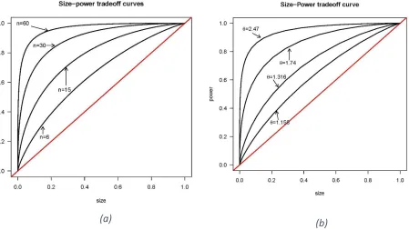
1. Given Ωk and σ2, for any matrix Q, the larger the number of units, the greater the power of the test, everything else being equal. Note that a larger n reduces the variance of T. As the sample size increases, the sampling distribution of T under the null and the alternative hypotheses is concentrated around θ. Fig.: 1(a) shows the size-power tradeoff curves of the test statistic T for different n with Q = Ik, rank(Ωk) = 4,
τ =M(ηi)
σ2 = 0.35. This means that on average, the randomness of the model is 35% of σ2. The plot shows the consistency and unbiasedness of the test.
2. Given Ωk, the larger the variance σ2, the closer θ is to one, and the lower the power of the test. Conversely, the smaller the variance, the farther θ is from one, and the greater the power of the test. Fig.:1(b) shows the size-power tradeoff curves of the test T for different values of θ and n = 7. The reciprocal of the parameter θ, θ−1= σ2/(σ2+ M(η
i)), may be viewed as a measure of the share of σ2 in ”total” variability. It ranges between zero and one. When data come from an LR model θ−1= 1, when at least one eigenvalue is greater than zero, θ−1< 1. The closer θ−1 is to zero, the stronger the evidence against an LR model. In applications θ−1 may have a more immediate interpretation than θ. Fig.:1(b) shows a share that moves from
θ−1= 1/1.158 = 0.86 to θ−1= 1/2.47 = 0.4.
3. Given σ2, if Ωk ⪰ 0 , M(ηi)
σ2 > 0, θ is greater than 1 and T deviates from 1. The farther M(ηi) is from zero, the greater T is and the stronger the evidence against an LR model. We recall that the magnitude of
M(ηi) =1
p
k
i=1 ηi depends both on the rank of Ωk (on how many eigenvalues are zero) and on the rank of the projector VQVQ+ given by the rank of the matrix Q (the denominator, p). The quantity M(η
i) ”appropriately” captures the randomness of parameters when it is ”true” arithmetic mean, that is, when
𝑟𝑎𝑛𝑘(Ωk) = 𝑟𝑎𝑛𝑘(VQVQ+). If the rank of Ωk is less than the rank of the projection matrix (information unknown in applications) the effect of randomness could be overlooked (undersized).
(a)
(b)
An important ”instrument” useful to define ”appropriately”M(ηi) could be the specification of the model. Let’s suppose that a matrix Zi (with rank q) of covariates is defined, then, implicitly we assume that
𝑟𝑎𝑛𝑘(Ωk) ≤ q. In this case there are two possible options for the choice of Q. We could ignore the additional information coming from Zi and set Q = Ik, or define a semi-orthogonal q × k matrix, Q such that Zi = XiQ′. If 𝑟𝑎𝑛𝑘(Ωk) = q, the projection of Zi on the kernel of X allows to construct a test statistic very close to FW and more powerful than a test computed with Q = Ik. If the rank of Ωk is less than q, the matrix Q does not allow to ”capture” the ”full” randomness. In this case M(ηi) is not a ”true” arithmetic mean, the number of non zero eigenvalues of the numerator is less than the denominator. Therefore, any attempt to improve the performance of the test goes through the definition of M(ηi) as a ”true” arithmetic mean. To achieve this goal we propose to define Q as a row vector. This approach produces a set of k test statistics (one for each column of the matrix Xi) that are analyzed within a multiple testing procedure.
5.3 A multiple-testing approach: the statistic 𝐓𝐁
The above analysis of M(ηi) suggests a way to improve the power of the test statistic T: define Q so that
M(ηi) is a ”true” arithmetic mean. The consequence of this approach is the computation of k test statistics, each of which tests the same null hypothesis, H0:Ωk = 0. To emphasize this column-by-column approach, the quantities T
and θ will be indicated as Tj, θj j = 1, … , k.Following, we compute a set of k correlated tests, Tj j = 1, … , k, which show the following features,
i. The expected value and the shape of Tj depend on the parameter θj which is similar (in value) for each individual test. As a consequence the statistics Tj show similar summary statistics (see Table 2).
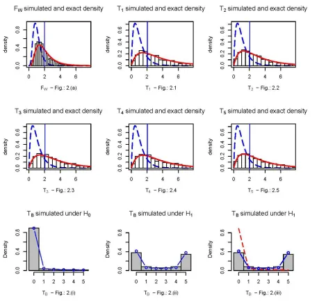
ii. They have the same distribution under the null hypothesis: Tj ∼ F n − 1, Nt− nk . Under the alternative hypothesis the funcional form is described in section 4.3 and depends on θj (the ”non-centrality parameter”). These parameters are close from each to the others (see Table 2). Figures 2.1 − 2.5 show the simulated Tj and the exact density functions under H0 (long dashed lines) and under the alternative hypothesis (solid line). iii. Both statistical powers (and p-values) are very close for each statistic Tj (see Table 1)
iv. All individual tests are more powerful than FW (see Table 1).
Therefore, given Tj, j = 1, … , k, the problem is how to summarize this set of statistics so that we reject the null hypothesis without losing the statistical power of the individual tests. At first we could proceed by computing the arithmetic mean T =1k ki=1Tj and then making inference with T. This approach is not analyzed, instead we deal with the problem of the ”synthesis” within a ”multiple testing” procedure.Let us transform the p-values associated with each individual tests Tj into k realizations of Bernoulli variables and denote with TB the number of rejections (p-value less than a level α) after performing the k tests individually. If Hi, i = 0,1 is true, then TB ∼ BB(k, γ, ϕ) whereBB . is for Beta Binomial, γ denotes the probability parameter and ϕ the over-dispersion parameter. The beta binomial distribution is analyzed by simulation using the HRQoL package of R-program Najera-Zuloaga et al. (2017) to estimate the parameters. We observed the following results:
i. All simulations show that the estimate of γ (by method of moments) is always equal to the arithmetic mean of the simulated power of the individual tests Tj. This leads us to state that the ”true” probability parameter is equal to the arithmetic mean of ”true” statistical powers. Following, we set γ =1k kj=1P(Tj > cv|Hj: θj ≥
1) where cv is the critical value equal for each statistic. Under H0, γ is known, equal to the probability of Type I error, γ = α. Under the alternative hypothesis it is unknown but as it is the arithmetic mean of the statistical powers of individual test it does not lose the power of the test.
ii. An analysis of the estimates of the overdispersion parameter is more complex. Our findings show two aspects: under H0 we estimate an intraclass correlation coefficient around 0.5, under H1 the larger is θj, the larger is the simulated ϕ with a magnitude around the arithmetic mean of θj. These observations induced us to set
ϕ =1
k
k
The above observations are highlighted in Table 3 and Figures 2. (i) − 2. (iii).
Therefore, provided that H0 is true, we reject the null hypothesis when TB is greater than or equal to the 1 − α percentile of the beta binomial distribution BB(k, 0.05,1). More precisely, with k = 5 we reject the null hypothesis if
TB > 2 = 0.0406. We can look at the Table 3 and evaluate the statistical power. It is equal to 5i=3P(TB = i|H1) =
0.482 wich is equal to a mean of the simulated power of the individual tests. Therefore, it is an estimate of the true Figure 2: - Fig.: 2. (a) and Fig.: 2.1 − 2.5 show simulated histogram of FW and Tj, j = 1, … ,5 under
power γ = 0.503.
Number
replic.= 1000
Number of units
n = 10 n = 20 n = 50 n = 100
Test Statistic
Statistical Power
FW 0.24 0.37 0.61 0.85
T1 0.37 0.57 0.83 0.99
T2 0.34 0.56 0.79 0.98
T3 0.36 0.59 0.84 0.99
T4 0.35 0.55 0.82 0.98
T5 0.36 0.56 0.80 0.99
Table 1: Statistical Power,
α = 0.05
,
rank
(
Ω
k) = 3
,
τ = 0.18
Test Statistics
T1 T2 T3 T4 T5 FW
Summary Statistics
2.5𝑡ℎ percentile 0.367 0.321 0.365 0.3758 0.329 0.5667
5𝑡ℎ percentile 0.5435 0.476 0.539 0.555 0.487 0.688
Median 2.778 2.456 2.749 2.807 2.568 1.779
Mean 3.558 3.151 3.52 3.581 3.321 2.05
95𝑡ℎ percentile 9.211 8.18 9.108 9.224 8.706 4.33
97.5𝑡ℎ percentile 11.253 9.989 11.13 11.26 10.65 5.112
θj 3.349 2.966 3.133 3.370 3.126 1.953 ϕ = 2.662
θj−1 0.298 0.337 0.302 0.297 0.319
True power 0.523 0.463 0.517 0.523 0.485 0.336 γ = 0.503
Simulated power 0.504 0.446 0.501 0.498 0.459 γ = 0.482
Table 2: Summary statistics of
T
jTB
TB Simulated BB(5,0.05,1) Simulated BB(5, γ, ϕ)
TB|H0 TB|H1
0 0.885 0.89 0.38 0.411
1 0.056 0.045 0.081 0.0624
2 0.019 0.024 0.058 0.045
3 0.014 0.0167 0.056 0.0446
4 0.014 0.013 0.082 0.0614
5 0.012 0.011 0.343 0.375
Table 3: Beta Binomial distribution of
T
B6 Conclusions
In the light of these results we believe that our two-stage approach based on a combinnation of a ”repeatable”
F −type test with a multiple testing approach may suggest a procedure for improving statistical power in linear mixed models. Future work should entail the refining of the second stage of the procedure by exploiting different ways for assessing the Bernoulli trials.
Appendix A Density and moments of the test statistic 𝐓
Let consider the following quadratic form T∗= tr V
Qp(n−1)σbb′ 2. obtained from (11) by replacing s2 with σ2. According to the assumptions of the model, T∗ has the same distribution as 1
(n−1)p
n−1
i=1 1 +σλi2 Zi2 where Zi2 are independent central χ2 random variables each with one degree of freedom; λ
i, i = 1, … , n − 1 are the eigenvalues of the product VQ VQ++ C I
n⊗Ωσ2k C′ (Mathai and Provost(1992) Section 3.1a. 2, singular case, p. 35).
When Ωk = 0, T∗ has a gamma distribution, G α =(n−1)p2 , β =(n−1)p2 and n − 1 p T∗ is distributed as a χ2 with (n − 1)p degrees of freedom.
When Ωk ⪰ 0, T∗ is a sum of gamma distributions each of which with same shape parameter, (n − 1)p/2, but r different scale parameters, 2 1 +λi
σ2 /((n − 1)p).
Then, the sample statistic T = σs22 T∗ has the same distribution as the random variable
W =d f T∗
d f s2/σ2
= df T∗
df s2/σ2 , df = Nt− nk (17)
where the numerator is a sum of (n − 1) gamma, G α = 1/2, βi = 2 1 +σλi2 df
(n−1)p , the denominator can be seen as a gamma, G α = df/2, β = 2 .
When Ωk = 0, W is the ratio of two chi-squared variates divided by the corresponding number of degrees of freedom, thus T ∼ F (n − 1)p, Nt− nk . If Ωk ⪰ 0 the distribution is more complex. Using the single gamma series representation proposed by Moschopoulos(1985) we can write the probability density function of W as
fT(w) =
∞
k=0
pkG(ρ + k, β1)
G df2, 2 (18)
where pk = Cδk, β1= mini{βi}, C = n−1
i=1 ββ1i αi
, ρ = n−1
j=1 αj and the coefficients δk can be obtained recursively by the formula
δ0 = 1
δk+1 =k+11 k+1i=1 j=1n−1αj 1 −ββ1 j
i
δk+1−i, k = 0,1,2, …
The expression (18) is the ratio of two independent gamma random variables then we can repropose the probability density of W as a generalized F-distribution (GF-distribution) getting,
fT(w) =
∞
k=0
pk GF ρ + k,df 2,
β1
2
where GF is for generalized F-distribution. Moments of T of order s are given by
E T𝑠 = ∞
k=0pk E XGFs where
E XGFs = (β
1/2)s Γ(ρ+k+s)Γ(γ−s)Γ(ρ+k)Γ(γ)
E(Ts) = (β1/2)s
(γ−1)…(γ−s)
∞
k=0 pk ρ + k s (19)
where (. )s is the Pochhammer symbol for rising factorial, γ = df/2.
References
Akaike, H. (1973) Information theory and an extension of the maximum likelihood principle. In Second international symposium on information theory (eds. H. Akaike, B. N. Petrov and F. Csaki), 267–281. Akadèmiai Kiadò. Demidenko, E., Sargent, J. and Onega, T. (2012) Random effects coefficient of determination for mixed and meta
analysis models. Communication in Statistics – Theory and Methods, 41(6), 953–969.
Demidenko, E. (2013) Mixed Models. Theory and application with R. 2nd ed. Hoboken, New Jersey, Wiley.
Drikvandi, R., Verbeke, G., Khodadadi, A. and Nia, V. (2013) Testing multiple variance components in linear mixed-effects models. Biostatistics, 14, 144–159.
Fitzmaurice, G., Lipsitz, S. and Ibrahim, J. (2007) A note on permutation tests for variance components in multilevel generalized linear mixed mdels. Biometrics, 63, 942–946.
Hui, F., Muller, S. and Welsh, A. (2019) Testing random effects in linear mixed models: another look at the F-test (with discussion). Australian and New Zealand Journal of Statistics, 61(1), 61–84.
Hunt, D., Cheng, C. and Pounds, S. (2009) The beta-binomial distribution for estimating the number of false rejections in microarray gene expression studies. Computational Statistics and Data analysis, 53, 1688–1700.
Jiang, J., Rao, J. S., Gu, Z. and Nguyen, T. (2008) Fence methods for mixed model selection. Ann. Statist., 36, 1669–1692.
Laird, N. M. and Ware, J. K. (1982) Random effect models for longitudinal data. Biometrics, 38, 963–974.
Laird, N. M. (2004) Chapter 5: Random effects and the linear mixed model, Volume 8 of Regional Conference Series in Probability and Statistics, 79–95. Beechwood OH and Alexandria VA: Institute of Mathematical Statistics and American Statistical Association. URL https://projecteuclid.org/euclid.cbms/1462106081 .
Mathai, A. M. and Provost, S. B. (1992) Quadratic forms in random variables: theory and applications. Marcel Dekker Inc.
Moschopoulos, P. G. (1985) The distribution of the sum of independent gamma random variables. Ann. Inst. Statist. Math., 37, Part A, 541–544.
Muller, S., Scealy, J. L. and Welsh, A. H. (2013) Model selection in linear mixed models. Statistical Science, 28, No. 2, 135–167.
Nagao, H. (1973) On some test criteria for covariance matrix. Annals of Statistics, 1, 700–709.
Najera-Zuloaga, J., Lee, D.J. and Arostegui, I. (2017) HRQoL: Health Related Quality of Life Analysis. URL https://CRAN.R-project.org/package=HRQoL . R package version 1.0.
Pillai, K. C. S. and Jayachandran, K. (1968) Power comparison of tests of equality of two covariance matrices based on four criteria. Biometrika, 55, 335–342.
Pillai, K. C. S. (1955) Some new test criteria in multivariate analysis. Ann. Mathem. Stat., No. 1, 26, 117–121.
Qiu, W. and Joe., H. (2015) clusterGeneration: Random Cluster Generation (with Specified Degree of Separation). URL https://CRAN.R-project.org/package=clusterGeneration . R package version 1.3.4.
Rocha, F. M. M. and Singer, J. M. (2017) Selection of terms in random coefficient regression models. Journal of Applied Statistics, DOI: 10.1080/02664763.2016.1273884.
Roy, S. (1953) On a heuristic method of test construction and its use in multivariate analysis. Annals of Mathematical Statistics, 24, 220–238.
R Core Team (2014) R: A Language and Environment for Statistical Computing. R Foundation for Statistical Computing, Vienna, Austria. URL http://www.R-project.org/.
Samuh, M., Grilli, L., Rampichini, C., Salmaso, L. and Lunardon, F. (2012) The use of prmutation tests for variance components in linear mixed models. Communications in Statistics- Theory and methods, 41, 3020–3029. Scheipl, F., Greven, S. and Kuechenhoff, H. (2008) Size and power of tests for a zero random effect variance or
polynomial regression in additive and linear mixed models. Computational Statistics and Data Analysis, 52, 3283–3299.
Searle, S. R. (1971) Linear Models. New York: Wiley.
Seely, J. and El-Bassiouni, Y. (1983) Applying Wald’s variance component test. The Annals of Statistics, 11, No 1, 197–201.
Sinha, S. (2009) Bootstrap tests for variance components in generalized linear mixed models. The Canadian Journal of Statistics, 37, 219–234.
Soetaert, K. and Herman, P. M. (2009) A practical Guide to Ecological Modelling. Using R as a Simulation Platform. Springer.
Theil, H. (1963) On the Use of Incomplete Prior Information in Regression Analysis. Journal of America Statistical Association, Vol. 58, 401–414.
Tibshirani, R. (1996) Regression shrinkage and selection via the lasso. Journal of Roy. Statist. Soc. Ser. B, 58, 267–288. Vaida, F. and Blanchard, S. (2005) Conditional Akaike information for mixed-effects models. Biometrika, 92 (2),
351–370.