JIEM, 2017 – 10(5): 853-886 – Online ISSN: 2013-0953 – Print ISSN: 2013-8423 https://doi.org/10.3926/jiem.2353
Using the Hybrid Fuzzy Goal Programming Model and Hybrid Genetic
Algorithm to Solve a Multi-Objective Location Routing Problem for
Infectious Waste Disposal
Narong Wichapa , Porntep Khokhajaikiat
Khon Kaen University (Thailand)
[email protected], [email protected]
Received: May 2017
Accepted: September 2017
Abstract:
Purpose: Disposal of infectious waste remains one of the most serious problems in the social and environmental domains of almost every nation. Selection of new suitable locations and finding the optimal set of transport routes to transport infectious waste, namely location routing problem for infectious waste disposal, is one of the major problems in hazardous waste management.
Design/methodology/approach: Case study, which involves forty hospitals and three candidate municipalities in sub-Northeastern Thailand, is divided into two phases. The first phase is to choose suitable municipalities using hybrid fuzzy goal programming model which hybridizes the fuzzy analytic hierarchy process and fuzzy goal programming. The second phase is to find the optimal routes for each selected municipality using hybrid genetic algorithm which hybridizes the genetic algorithm and local searches including 2-Opt-move, Insertion-move and λ-interchange-move.
Originality/value: The novelty of the proposed methodologies, hybrid fuzzy goal programming model, is the simultaneous combination of criteria in order to choose new suitable locations, and the hybrid genetic algorithm can be used to determine the optimal routes which provide a minimum number of vehicles and minimum transportation cost under the actual situation, efficiently.
Keywords: multi-objective facility location problem, fuzzy analytic hierarchy process; fuzzy goal programming model, hybrid genetic algorithm, infectious waste disposal, multi-criteria decision making, location routing problem
1. Introduction
illegal disposal in inappropriate places. Hence the Thai government has set up a policy to encourage the construction of new disposal facilities at areas of potential municipalities, in order to address the abovementioned problems and increase the efficiency of infectious waste disposal. These disposal facilities must be able to serve nearby hospitals and at the same time must reduce economic, environmental, health, and social factors. In order to achieve maximum benefit, new disposal facilities need to be planned along with suitable transport routes which provide the lowest transportation cost in accordance with the due date time. Therefore, building new, suitable, disposal facilities and finding the transport routes for infectious waste disposal more effectively is becoming an issue that is particularly important to consider.
Community hospitals, with forty hospitals in sub-Northeastern Thailand, are one type of public hospital that has often found the abovementioned problems, because they are far from the existing disposal facilities of outside agencies. To address such problems, the government has set policies to locate the new sites for infectious waste disposal at areas of potential municipalities. Selecting new suitable sites in this case is a complex problem which is difficult to address using any existing techniques alone, because there are relevant factors which must be considered, including infrastructure, geological, environmental, social and cost factors. Certainly, all factors must be considered simultaneously in designing an optimal transportation network. Finally, in order to achieve maximum benefit, we need to find suitable transport routes which provide minimum transportation cost for each selected municipality.
Genetic algorithm (GA) is one of various meta-heuristic algorithms which are often used to solve the VRPs in the literature because it is a simple, flexible and powerful algorithm to solve NP-hard problems. However, in order to increase the efficiency of this algorithm, a new hybrid genetic algorithm (hybrid GA) is developed to solve the VRP in this case study, instead of the traditional GA. The major difference between the traditional GA and the hybrid GA in this case is that three local searches (2-Opt-move, Insertion-move and λ-interchange-move) are added to increase the efficiency of the algorithm. This is the major reason why hybrid GA is chosen as a suitable algorithm for solving the VRP in this paper.
The rest of the paper is organized as follows. Sections 2, 3 and 4 are Literature review, Methodology and Application of the proposed methodology respectively, and finally, Section 5 is the Conclusion.
2. Literature Review
3. Methodology
The solution approach for this case consists of the following stages. (i) The first phase of this research is to select suitable municipalities for infectious waste disposal from candidate municipalities, for which location selection in this case is a complex problem, a multi-objective facility problem. The HFGP model is formed in the first phase by combining FAHP and FGP models in order to achieve the lowest total cost and maximum total priority weight. (ii) After that, the VRP model and hybrid GA are used in the second phase in order to achieve the lowest transportation cost/minimum total distance by using the optimization techniques with LINGO13 and Visual studio 2015 (C++) respectively.
The details of selecting the new suitable municipalities and finding the suitable transport routes for minimizing transportation cost/minimizing total distance are as follows:
• Define the most important criteria for selection of locations for infectious waste disposal,
• Evaluate the global priority weights for each candidate municipality using FAHP,
• Formulate and compute a HFGP model,
• Select the new suitable municipalities for infectious waste disposal.
• Build and compute the VRP model using an optimization technique (LINGO13) and meta-heuristic technique with Visual studio 2015 (hybrid GA with C++), and
• Select the optimal routes for each selected municipality.
3.1. FAHP
From the literature reviewed, FAHP is a flexible and powerful tool to solve MADM problems. Hence, using FAHP should make a suitable approach to evaluate the global priority weights of each candidate municipality, in order to take these weights into a HFGP model in Section 3.2. In this paper, we calculated the priorities weights of elements in each level of hierichy via the geometric means method of Buckley (1985) and Buckley, Feuring and Hayashi (2001); see also in similar papers of Cebeci (2009) and Meixner (2009). In this paper, the fuzzy arithmetic operations on triangular fuzzy numbers (TFNs) can be expressed as follows:
Addition: F1F2 = (l1 +l2, m1 +m2, u1 +u2) (1)
Multiplication: F1F2 = (l1 ·l2, m1 ·m2 ·m2, u1 ·u2) (2)
Division: F1/F2 = (l1 /u2, m1 /m2, u1 /l2) (3)
Reciprocal: F1–1 = (1/u1, 1/m1, 1/l1) (4)
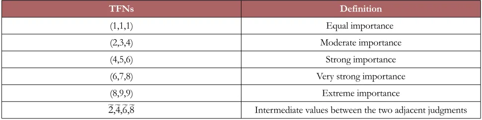
where l1 and l2 are the least possible value; m1 and m2 are modal value and u1 and u2 are highest possible value respectively. F1 and F2 are two TFNs; TFNs will be applied in order to compare a priority scale between criteria/elements as shown in Table 1.
TFNs Definition
(1,1,1) Equal importance
(2,3,4) Moderate importance
(4,5,6) Strong importance
(6,7,8) Very strong importance
(8,9,9) Extreme importance
Intermediate values between the two adjacent judgments
Table 1. The 9 - point scale of TFNs
3.1.1. Construct the Hierarchy
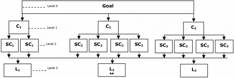
The relevant decision factors can be defined by asking questions to experts questions about which criterion is more important with regard to the goal. After that, these factors are decomposed into a multi-level hierarchical structure, as shown in Figure 1. At level “0”, the goal is to select new suitable municipalities for infectious waste disposal. At level “1”, the criteria are C1, C2, C3, at level “2”, the sub-criteria are SC11, SC12, ..., C34, and at level “3”, the candidate municipalities are L1, L2 and L3.
Figure 1. Multi-level hierarchy for selecting locations for infectious waste disposal
3.1.2. Construct the Comparison Matrices of Each Decision Maker
The comparison matrices of each decision maker k can be constructed using TFNs in Table 1. After that, integrating the comparison matrices from all experts using the fuzzy geometric mean method (Dong & Cooper, 2016; Meixner, 2009; Wichapa & Khokhajaikiat, 2017) is as shown in Equation (5).
(5)
Where is a aggregated comparison matrix of k decision makers, and is the
triangular fuzzy numbers of the kth decision maker.
3.1.3. Estimate Priority Weights of Each Level
And
(7)
The fuzzy priority weights have to be defuzzified, which can be converted to crisp priority weights using Equation (8) (Meixner, 2009; Tsaur, Chang & Yen, 2002).
(8)
3.1.4. Check for Consistency Ratio (CR) Values
1. Defuzzify aggregated comparison matrix and then multiply the crisp comparison matrix by the crisp priority weight vector.
2. Divide the weighted sum vector with criterion weight in step 1; average weighted sums (wi) will be
obtained for each row i for the calculation in this step.
3. Compute λmax by Equation (9).
(9)
4. Compute the consistency index (CI ) and CR by Equation (10).
CI = (λmax – n)/(n –1)and CR = CI/RI ≤ 0.10 (10)
A CR value of 0.10 or less is accepted as a good consistency measure. If the value exceeds 0.10, it is indicative of inconsistent judgment, and it should be revised as shown in related papers of researchers (Cebeci, 2009; Meixner, 2009; Wichapa & Khokhajaikiat, 2017).
3.1.5. Compute the Final Priority Weights for Each Alternative
3.2. HFGP Model
The multi-objective facility location problem model (MOFLP model) for infectious waste disposal is formulated to select multi-size incinerators and multiple municipalities. In addition, this model is formulated to respond to two objectives, minimize total cost and maximize total priority weight. Details of the mathematical model of this problem are shown below.
Indices:
i is the index of each municipality, I = 1,2,..,m, (m = 3).
j is the index of each hospital, j = 1,2,..,n, (n = 40).
k is the size of each incinerator, k = 1,..,K, (K = 2).
Parameters:
fk is the facility cost (baht/week).
ok is the operating cost (baht/ week).
cij is the transportation cost between municipality i and hospital j (baht/week)
dtij is the real distance between municipality i and hospital j (km).
u is the unit transportation cost (baht/km).
sk is the size of each incinerator i.
dj is the demand of hospital j (kg/week).
wi is the global priority weights of municipality i.
DT is the maximum allowable distance.
Decision variables:
Xij is a binary decision variable; Xij = 1 if the hospital j is served by the municipality I, Xij = 0 otherwise.
Yi is a non-negative integer decision variable; Yi = 1 if municipality i is opened, Yi = 0 otherwise.
Zik is a binary decision variable; Zik = 1 if the municipality i is opened by selecting incinerator k, Zik = 0
otherwise.
Objective function:
(12)
Subject to:
(13)
(14)
(15)
(16)
dtij · Xij ≤ DT i (i = 1 ....m) j (i = 1 ....n) (17)
Xij {0,1} (18)
Yi {0,1} (19)
Zi,k {0,1} (20)
In this paper, the first objective function of the MOFLP model is to minimize total cost as shown in Equation (11), and the second objective function is to maximize total location weight as shown in Equation (12). Equation (13) ensures that the demand of each hospital j is fulfilled. Equation (14) expresses that the service prepared by a site cannot exceed its capacity. Equation (15) expresses that the sum of the service provided by sites cannot exceed the sum of its capacities and Equation (16), the selected municipalities must use only k-size incinerators. Equation (17) expresses that each travel distance from point i to point j cannot exceed the maximum acceptable distance. Equations (18), (19) and (20) are binary.
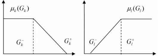
In this case study, the target value associated with each goal could be fuzzy, and both goal 1 (G1) and goal 2 (G2) might not be completed simultaneously under the system constraints. In order to address this problem, based on Zimmermann (1978), he expressed objective functions Gj, j = 1, 2..q by fuzzy sets
(21)
(22)
and are ideal solutions, minimum values of goal Gk and maximum value of goal Gl respectively.
and Gl are non-ideal solutions, the maximum value of goal Gkand the minimum value of goal Gl
respectively. Linear membership functions μ(Gj(x)) are shown in Figure 2.
Figure 2. Objective function as fuzzy numbers of min Gk and max Gl
The target of two objectives of the multi-objective facility location problem model for location selection for infectious disposal is fuzzy values, and these objectives can be written for fuzzy goal programming (FGP) as follows:
(23)
(24)
Objective function:
Max G = λ (25)
Subject to:
wG1λ ≤ (max G1 – G1)/(max G1 – min G1) (26)
wG2λ ≤ (G2 – min G2)/(max G2 – min G2) (27)
(28)
(29)
where Equation (25) is an objective function as maximization of the lambda value. Equations (26) and (27) are fuzzy objective constraints. Equation (28) gives system constraints, which refers to Equations (13)-(20) of the MOFLP model. In Equation (29), wGiare priority weights of each goal according to
experts’ opinions. The optimal solution of the HFGP model can be solved by LINGO 13.
3.3. VRP Model for Infectious Waste Disposal
After obtaining the suitable municipalities from computing the HFGP model in Section 3.1, the municipalities that have been selected as disposal centers for infectious waste disposal must be assigned the best routes to achieve the lowest total distance. Details of the VRP model are as follows.
Indices:
The VRP model for infectious waste disposal may be defined as the following graph theoretic problem. Let G = (N, A) be a complete graph where N = {1, 2, 3, …, n} is a set of hospitals and municipality. A is the arc set, pair of nodes (i, j). N=2, 3, 4, …, n is a set of hospitals, whereas N = 1 is a selected municipality/a single depot. K is a set of identical vehicles, which is available at the municipality.
Parameters:
dtijis actual distance from node i to j (km) that is symmetrical (dtij= dtji)
N is a set of hospitals and municipalities, N = {1, 2, 3, ..., n}.
qkis the capacity of each vehicle k (kg).
dj is the amount of waste collected from hospital j (kg).
tijis the travel time from node i to j (min.) that is symmetrical (tij= tji).
D is the maximum permitted travel time per vehicle (min.). Each vehicle travels from node i to j at a speed of 60 kilometers per hour (tij= dtij).
Decision variables:
Xijk =1, if vehicle k drives from hospital i to j, Xijk = 0, otherwise.
Zk =1, if vehicle k is used to service hospitals, Zk = 0 otherwise.
Objective function:
(30)
Constraints:
(31)
(32)
(33)
(34)
(35)
(36)
(37)
Xijk{0, 1} i N, j N, k K (39)
Zk{0, 1} (40)
Yi – Yj + N · Xijk ≤ N – 1 i = 2, 3, 4, …,n;j = 2, 3, 4, …,n; i j; k K (41)
The objective is to minimize the total distance, as shown in Equation (30). Equation (31) guarantees that the number of arcs from node i and node j does not exceed n nodes. Equation (32) and Equation (33) guarantee that a vehicle must start at a selected municipality to hospitals only once. Equation (34) guarantees that if a vehicle visits a hospital j, it also leaves that hospital j. Equations (35) and (36) guarantee that all hospitals are visited only once. Equation (37) guarantees that the amount of infectious waste of each hospital will be fulfilled by vehicles k but does not exceed the capacity of the vehicle itself. Equation (38) ensures that every vehicle k cannot travel more than the tour length restriction. Equation (39) and Equation (40) guarantee the decision variables xijk and zk to be binary decision variables.
Equation (41) guarantees that there will be no sub tours.
In this case study, hybrid GA will be used to solve the VRP model for infectious waste disposal in this case as shown in the next section.
3.4. Hybrid GA
on relevant parameters such as probability of crossover, probability of mutation, population size, repetition number, and algorithm.
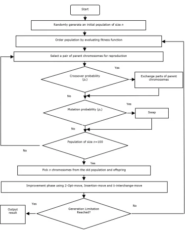
A hybrid genetic algorithm (Hybrid GA), which integrates GA and three local searches (insertion-move, 2-opt-move and λ-interchange-move), was proposed to solve the VRP in this case. The first objective of the hybrid GA is to minimize the number of vehicles (NV) and the second objective is to minimize the total distance (TD), under the limits of existing resources. The algorithm is shown in Figure 3.
Figure 3 can be described as follows. Let n be the size of the population at each generation. An initial population will be randomly generated until the size is equal to n. After that, the chromosomes in the initial population are sorted by fitness, and then a pair of chromosomes is randomly chosen for mating using the ranking-based selection of Correa et al. (Correa, Steiner, Freitas & Carnieri, 2001), as shown in Equation (42).
(42)
OS is an ordered list of solutions sorted by fitness.
P is the position in the OS to be selected as the chromosome Sp.
rnd (M) is a random distribution in the range 0 to M-1.
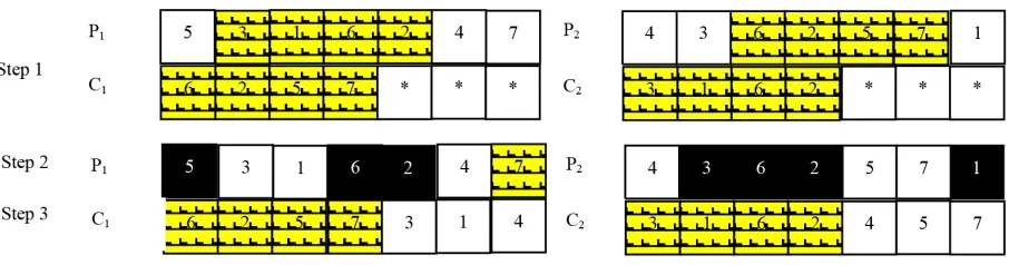
After that, with crossover probability (pc), exchange parts of a pair of parents and create two offspring as
shown in Figure 4.
Figure 4. Crossover procedure
• Randomize indices cut1 and cut2, where cut1 < cut2
• Step 1: Copy hospitals in parent-1 (P1) from indices cut1 to cut2 to child-2 (C2) starting at index 0. Also hospitals in parent-2 (P2) from indices cut1 to cut2 to child-1 (C1) starting at index 0.
• Step 2: mask hospitals in P1 that already are contained in C1 and also mask hospitals in P2 that already are contained in C2.
• Step 3: fill hospitals that unmask in C1 to P1 and C2 to P2.
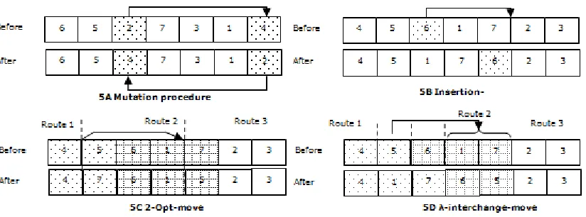
In the mutation procedure, with the mutation probability pm, hospitals in the two offspring chromosomes
be combined and n chromosomes picked to be the new population using fitness. If a new chromosome is better than any chromosome in the current population, the new chromosome will be included and the worst one in the current population will be removed. Finally, the chromosomes in the new population will be improved by three local searches, insertion-move, 2-opt and λ-interexchange, as shown in Figure 5B, Figure 5C and Figure 5D respectively.
Figure 5. Mutation and three local searches (Insertion, 2-Opt and λ-interchange)
The selection is still a rank-based selection and selects chromosomes n times for each local search. This procedure is repeated until the stopping criteria are satisfied. Implementation and computational results of the hybrid GA are reported in the next section.
4. Application of the Proposed Methodology
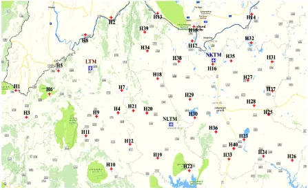
Figure 6. The transportation network of the candidate municipalities and hospitals
4.1. Estimate the Priority Weights of Municipalities Using FAHP
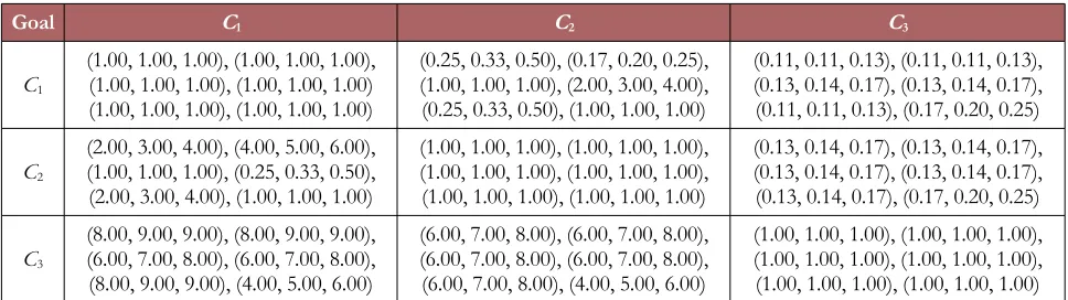
Goal C1 C2 C3
C1
(1.00, 1.00, 1.00), (1.00, 1.00, 1.00), (1.00, 1.00, 1.00), (1.00, 1.00, 1.00) (1.00, 1.00, 1.00), (1.00, 1.00, 1.00)
(0.25, 0.33, 0.50), (0.17, 0.20, 0.25), (1.00, 1.00, 1.00), (2.00, 3.00, 4.00), (0.25, 0.33, 0.50), (1.00, 1.00, 1.00)
(0.11, 0.11, 0.13), (0.11, 0.11, 0.13), (0.13, 0.14, 0.17), (0.13, 0.14, 0.17), (0.11, 0.11, 0.13), (0.17, 0.20, 0.25)
C2
(2.00, 3.00, 4.00), (4.00, 5.00, 6.00), (1.00, 1.00, 1.00), (0.25, 0.33, 0.50), (2.00, 3.00, 4.00), (1.00, 1.00, 1.00)
(1.00, 1.00, 1.00), (1.00, 1.00, 1.00), (1.00, 1.00, 1.00), (1.00, 1.00, 1.00), (1.00, 1.00, 1.00), (1.00, 1.00, 1.00)
(0.13, 0.14, 0.17), (0.13, 0.14, 0.17), (0.13, 0.14, 0.17), (0.13, 0.14, 0.17), (0.13, 0.14, 0.17), (0.17, 0.20, 0.25)
C3
(8.00, 9.00, 9.00), (8.00, 9.00, 9.00), (6.00, 7.00, 8.00), (6.00, 7.00, 8.00), (8.00, 9.00, 9.00), (4.00, 5.00, 6.00)
(6.00, 7.00, 8.00), (6.00, 7.00, 8.00), (6.00, 7.00, 8.00), (6.00, 7.00, 8.00), (6.00, 7.00, 8.00), (4.00, 5.00, 6.00)
(1.00, 1.00, 1.00), (1.00, 1.00, 1.00), (1.00, 1.00, 1.00), (1.00, 1.00, 1.00), (1.00, 1.00, 1.00), (1.00, 1.00, 1.00)
Table 2. The comparison matrix of criteria with respect to goal by the six experts
Combined
comparison matrix C1 C2 C3 wi CR
C1 (1, 1, 1) (0.52, 0.64, 0.79) (0.12, 0.13, 0.15) (0.08, 0.09, 0.12) 0.10
0.03 C2 (1.26, 1.57, 1.91) (1, 1, 1) (0.13, 0.15, 0.18) (0.11, 0.13, 0.17) 0.13
C3 (6.48, 7.50, 8.09) (5.61, 6.62, 7.63) (1, 1, 1) (0.65, 0.79, 0.95) 0.77
Table 3. The combined comparison matrix of six decision makers
Candidate municipalities Global priority weights (wi)
Nongbua Lamphu Town Municipality (NLTM) 0.55
Nong Khai Town Municipality (NKTM) 0.21
Loei Town Municipality (LTM) 0.24
Table 4. Global priority weights of candidate municipalities
4.2. Compute the Suitable Locations Using HFGP Model
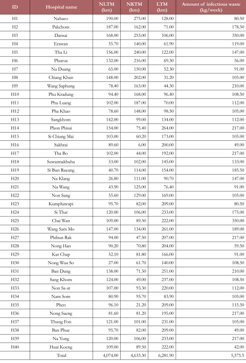
The wi of each candidate municipality are found based on Section 4.1 to be w1 (global priority weight of NLTM) = 0.55, w2 (global priority weight of NKTM) = 0.21 and w3 (global priority weight of LTM) = 0.24. In order to solve the MOFLP in this case, set wG1>wG2 according to experts’ opinions; the sensitivity analysis of the HFGP was also performed for different levels of objective weights. The actual distance matrix and demands of three candidate municipalities and forty hospitals are shown in Table 5 as
dj, dtij. The values of u and DT are 4.3 baht/km and 240 km respectively. In Table 6, fk (k = 1 and k = 2)
are 13,248 and 24,395 baht per week, and ok are 69,090 and 130,508 baht per week respectively. The
values of sk are about 3,000 and 6,000 kg per week. The data set for membership functions of each goal
ID Hospital name NLTM(km) NKTM(km) LTM(km) Amount of infectious waste(kg/week)
H1 Nahaeo 190.00 275.00 128.00 80.50
H2 Pakchom 187.00 162.00 71.00 178.50
H3 Dansai 168.00 253.00 106.00 350.00
H4 Erawan 55.70 140.00 61.90 119.00
H5 Tha Li 156.00 240.00 122.00 147.00
H6 Phurua 132.00 216.00 69.30 56.00
H7 Na Duang 65.00 150.00 52.30 91.00
H8 Chiang Khan 148.00 202.00 31.20 105.00
H9 Wang Saphung 78.40 163.00 44.30 210.00
H10 Phu Kradung 94.40 168.00 96.40 108.50
H11 Phu Luang 102.00 187.00 70.00 112.00
H12 Pha Khao 78.60 148.00 98.50 105.00
H13 Sangkhom 142.00 99.00 134.00 112.00
H14 Phon Phisai 154.00 75.40 264.00 217.00 H15 Si Chiang Mai 103.00 60.20 173.00 105.00
H16 Sakhrai 89.60 6.00 200.00 49.00
H17 Tha Bo 102.00 44.00 192.00 217.00
H18 Suwannakhuha 53.00 102.00 145.00 133.00 H19 Si Bun Rueang 40.70 114.00 154.00 185.50
H20 Na Klang 26.80 111.00 90.70 147.00
H21 Na Wang 43.90 125.00 76.40 91.00
H22 Non Sang 55.60 129.00 169.00 105.00
H23 Kumphawapi 95.70 82.00 209.00 80.50
H24 Si That 120.00 106.00 233.00 175.00
H25 Chai Wan 109.00 89.50 222.00 350.00
H26 Wang Sam Mo 147.00 134.00 261.00 189.00
H27 Phibun Rak 94.00 47.50 207.00 217.00
H28 Nong Han 90.20 70.80 204.00 59.50
H29 Kut Chap 52.10 81.80 166.00 91.00
H30 Nong Wua So 27.00 61.70 140.00 108.50
H31 Ban Dung 138.00 71.50 251.00 210.00
H32 Sang Khom 124.00 49.00 237.00 108.50
H33 Non Sa-at 107.00 93.30 220.00 112.00
H34 Nam Som 80.90 95.70 83.90 105.00
H35 Phen 96.10 21.20 209.00 115.50
H36 Nong Saeng 81.60 81.20 195.00 217.00
H37 Thung Fon 121.00 101.00 231.00 105.00
H38 Ban Phue 95.70 82.00 209.00 49.00
H39 Na Yung 120.00 106.00 233.00 217.00
H40 Huai Koeng 109.00 89.50 222.00 42.00
Details of the cost (baht/week)
Size of incinerator (kg/week)
3,000 6,000
1. Facility cost 1.1 Incinerator 1.2 Landfill 1.3 Storage
1.4 Infectious waste tank 1.5 Cleaning system 1.6 Emergency generator
1,918 479.5 6,902 1,725.5 115.5 2,107 3,836 959 13,811 3,451 231 2,107
Total facility cost (baht/day) 13,248 24,395
2. Operating cost per day 2.1 Labor cost
2.2 Maintenance costs (6% of incinerator) 2.3 Cost of measuring air pollution 2.4 Cost of IWD (3.3 Baht/kg )
51,026.5 1,151.5 7,672 9,240 102,053 2,303 7,672 18,480
Total operating cost (baht/day) 69,090 130,508
Table 6. Details of the cost
µ = 0 µ = 1 µ = 0
Min. total cost, G1 – 172,421.2 495,848.3
Max. total weight, G2 0.45 1 –
Table 7. Data set for membership functions
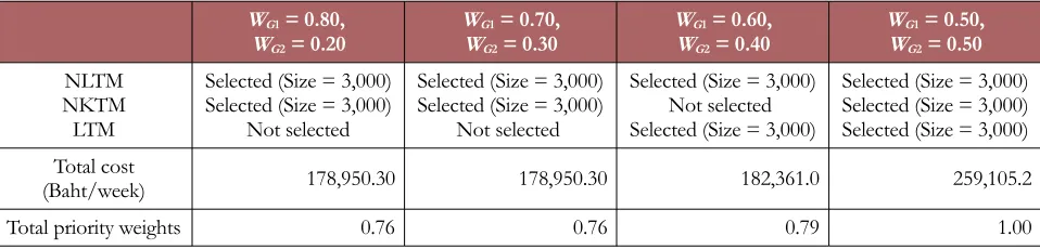
These relevant parameters were taken to place into the HFGP model (Equation 25 to 29). Afterward, the LINGO 13 software was applied, and the optimal solutions for different objective weights were as shown in Table 8.
WG1 = 0.80,
WG2 = 0.20
WG1 = 0.70,
WG2 = 0.30
WG1 = 0.60,
WG2 = 0.40
WG1 = 0.50,
WG2 = 0.50
NLTM NKTM LTM
Selected (Size = 3,000) Selected (Size = 3,000)
Not selected
Selected (Size = 3,000) Selected (Size = 3,000)
Not selected
Selected (Size = 3,000) Not selected Selected (Size = 3,000)
Selected (Size = 3,000) Selected (Size = 3,000) Selected (Size = 3,000) Total cost
(Baht/week) 178,950.30 178,950.30 182,361.0 259,105.2
Total priority weights 0.76 0.76 0.79 1.00
Table 8. Sensitivity analysis for different values of objective’s weights
same time, the number of locations and total cost have an increasing trend. Finally, the optimal solutions from the sensitivity analysis for different values of objective weights were offered to the four decision makers. The four decision makers made the decision to choose the NLTM and NKTM as suitable municipalities for infectious waste disposal, with the following reasons: “Although total priority weight of selected municipalities is not equal to the maximum predefined value (Target = 1), the total cost is a minimum total cost. If we choose the others, the total cost will be very high, which is not according to experts’ opinions (wG1 > wG2)”
The results show that the suitable candidate municipalities were NLTM and NKTM (selected by
wG1 = 0.70 and wG2 = 0.30). It can decrease the total cost by selection of NLTM and LTM by about 3,410.7 baht/week. Although the weight of NKTM was slightly lower than the weight of LTM, by about 0.03, the total cost objective was achieved using the new proposed model. Details of optimal solution of HFGP model are shown in Table 9.
Opened location Size of location
(kg/week) Hospitals
NLTM 3,000 H1, H3, H4, H5, H6, H7, H8, H9, H10, H11, H12,H18,H19, H20, H21, H22, H29, H30, H34, H36
NKTM 3,000 H2, H13, H14, H15, H16, H17, H23, H24, H25, H26, H27,H28, H31, H32, H33, H35, H37, H38, H39, H40
Total cost = 178,950.30 baht/week Total priority weight = 0.76
Table 9. Optimal solution of HFGP model
Therefore, this model can lead to the selection of new suitable locations for infectious waste disposal by considering both tangible factors and intangible factors simultaneously. In addition, the decision makers believed that our work can provide essential support for decision makers in the assessment of infectious waste disposal problems, in this case study and other areas of Thailand and, they also believe that the proposed methodology can be applied to other complex problems.
4.3. Find the Routes for Each Selected Municipality Using Hybrid GA
respectively. Actual distance matrices (dtij) and dj of each selected municipality are shown in actual distance
matrices of NLTM and NLTM, see details in Appendix A. The experiment was performed on a computer with the following characteristics: An Intel® Core™ i5-4210U processor Dual-core operating at 1.70 GHz with 8 GB of RAM, and Windows 8.1 operating system. The capacity of all vehicles (qk) is
equal to 1, 3 and 6 ton respectively. Each vehicle travels from node i to j at a constant speed of 60 kilometers per hour so the maximum permitted travel time per vehicle (D) is equal to 480 minutes according to the experts’ opinions. The input parameters for the experimentation in hybrid GA were made with an initial population of 100 individuals and 10 generations, and hybrid GA was tested to solve the actual problems using Visual Studio 2015 (C++). The probability for genetic operator in hybrid GA were set to be pc = 0.8 and pm = 0.3. The obtained results of each vehicle capacity are compared with
computational results using LINGO13 based on the VRP model in Section 4.3, as shown in Table 10.
From Problem 1.1 (N = 5), Problem 1.2 (N = 10), Problem 1.3 (N=15) and Problem 1.4 (N = 20), NLTM has been selected as a disposal center which needs to service 4 hospitals (H1, H3, H4, H5), 9 hospitals (H1, H3, H4, H5, H6, H7, H8, H9, H10), 14 hospitals (H1, H3, H4, H5, H6, H7, H8, H9, H10, H11, H12, H18, H19) and 20 hospitals (H1, H3, H4, H5, H6, H7, H8, H9, H10, H11, H12, H18, H19, H20, H21, H22, H29, H30, H34, H36) respectively. From Problem 2.1 (N = 5), Problem 2.2 (N = 10), Problem 2.3 (N = 15) and Problem 2.4 (N = 20), NKTM has been selected as a disposal center which needs to service 4 hospitals (H2, H13, H14, H15), 9 hospitals (H2, H13, H14, H15, H16, H17, H23, H24, H25), 14 hospitals (H2, H13, H14, H15, H16, H17, H23, H24, H25, H26, H27, H28, H31, H32) and 20 hospitals (H2, H13, H14, H15, H16, H17, H23, H24, H25, H26, H27, H28, H31, H32, H33, H35,H37, H38, H39,H40) respectively.
Vehicle
capacity Data set Number ofhospitals
LINGO13 Hybrid GA
Number of vehicles/routes (NV/NR) Total distance (TD) Computatio nal times (hh, mm, ss)
Number of vehicles/routes (NV/NR) Total distance (TD) Deviation 1 ton
Prob. 1.1 4 hospitals. 1 405.6 00:00:01 1 405.6 0%
Prob. 2.1 4 hospitals. 1 427.4 00:00:01 1 427.4 0%
Prob. 1.2 9 hospitals. 2 703.4 00:16:21 2 703.4 0%
Prob. 2.2 9 hospitals. 2 672.5 00:01:35 2 672.5 0%
Prob. 1.3 14 hospitals. 2 832.3 48:00:00 2 832.3 0%
Prob. 2.3 14 hospitals. 3 842.3 48:00:00 3 842.3 0%
Prob. 1.4 Actual casefor NLTM 3 1,149.5 48:00:00 3 1,149.5 0%
Prob. 2.4 Actual casefor NKTM 3 987.6* 48:00:00 3 987.6 0%
2 tons
Prob. 1.1 4 hospitals. 1 405.6 00:00:01 1 405.6 0%
Prob. 2.1 4 hospitals. 1 427.4 00:00:01 1 427.4 0%
Prob. 1.2 9 hospitals. 2 703.4 00:37:27 2 703.4 0%
Prob. 2.2 9 hospitals. 2 672.5 00:01:41 2 672.5 0%
Prob. 1.3 14 hospitals. 2 831.7 48:00:00 2 831.7 0%
Prob. 2.3 14 hospitals. 2 752.9 48:00:00 2 752.9 0%
Prob. 1.4 Actual casefor NLTM 3 1,129.8 48:00:00 3 1,129.8 0%
Prob. 2.4 Actual casefor NKTM 2 880.8 4800:00 2 880.8 0%
3 tons
Prob. 1.1 4 hospitals. 1 405.6 00:00:01 1 405.6 0%
Prob. 2.1 4 hospitals. 1 427.4 00:00:01 1 427.4 0%
Prob. 1.2 9 hospitals. 2 703.4 00:37:27 2 703.4 0%
Prob. 2.2 9 hospitals. 2 672.5 00:01:41 2 672.5 0%
Prob. 1.3 14 hospitals. 2 831.7 48:00:00 2 831.7 0%
Prob. 2.3 14 hospitals. 2 752.9 48:00:00 2 752.9 0%
Prob. 1.4 Actual casefor NLTM 3 1,129.8 48:00:00 3 1,129.8 0%
Prob. 2.4 Actual casefor NKTM 2 880.8 4800:00 2 880.8 0%
Table 10. Comparison of solutions using LINGO13 and hybrid GA
Municipality
name Vehicle size (Baht/week)Vehicle cost Transportation cost(Baht/week) (Baht/week)Total cost
NLTM
1 ton 3,835.62 (NV = 1) 1,149.5 × 4.3 = 4,942.85 8,778* 2 ton 5,753.43 (NV = 1) 1,129.8 × 4.3 = 4,858.14 10,612 3 ton 7,671.23 (NV = 1) 1,129.8 × 4.3 = 4,858.14 12,529
NKTM
1 ton 3,835.62 (NV = 1) 987.6 × 4.3 = 4,246.68 8,082*
2 ton 5,753.43 (NV = 1) 880.8 × 4.3 = 3,787.44 9,541
Disposal
centers (using vehicle capacity of 1 ton)Transport routes Distance(km) Amount of infectious waste (kg)
NLTM
Route 1 for Monday:
NLTM, H22, H19, H12, H10, H11, H9, H21, NLTM 331.1 917.0
Route 2for Wednesday:
NLTM, H7, H8, H5, H1, H3, H6, H4, NLTM 476.4 948.5
Route 3for Friday:
NLTM, H20, H34, H18, H29, H36, H30, NLTM 342.0 801.5
Total 1,149.5 2,667.0
NKTM
Route 1 for Monday:
NKTM, H35, H27, H28, H26, H24, H23, H40, H33, NKTM 337.6 990.5 Route 2for Wednesday:
NKTM, H38, H39, H2, H13, H15, H17, H16, NKTM 365.1 927.5
Route 3for Friday:
NKTM, H25, H37, H31, H32, H14, NKTM 284.9 990.5
Total 987.6 2,908.5
Table 12. Details of computational results for the actual problem using hybrid GA
As seen in Tables 11 and 12, in order to minimize the number of vehicles and transportation costs according to the decision makers’ opinions, a capacity of 1 ton was selected as a suitable size for NLTM and NKTM because it provides the lowest total cost (vehicles and transportation costs), and then it has been planned to pick up the infectious waste on Monday (Route 1), Wednesday (Route 2) and Friday (Route 3) for each selected municipality. Therefore, the proposed hybrid GA can lead to providing the lowest total cost under this actual case study, according to decision makers’ opinions.
5. Conclusion
In this study, the location routing problem, which is a complex problem, is handled within two phases consisting the multi-objective facility location problem to find a suitable new municipality for infectious waste disposal and the vehicle routing problem to analyze transport routes for the newly selected municipality, which aims to minimize transportation cost/total distance.
In the first phase, multi-objective facility location problem is considered with both quantitative and qualitative objectives. HFGP model is proposed to solve this complex problem.
municipalities among alternative municipalities for infectious waste disposal. The results show that NLTM and NKTM are two suitable locations. HFGP model enhances minimum total cost and the highest priority weight. In second phase, hybrid GA model is proposed to solve VRP. Firstly, LINGO13 was used to solve the VRP model in order to compare with hybrid GA.
The results show that the selected municipalities were assigned for infectious waste pickup efficiently using minimum number of vehicles and minimum total cost.
The major advantages of the proposed methodology are that the HFGP model can guide selection of a new suitable municipality by considering subjective and objective criteria simultaneously, and the hybrid GA can find the suitable transport routes, which require the minimum number of vehicles and minimum total cost, efficiently. These approaches are simple but powerful, and are flexible for decision makers to limit costs and environmental impacts. The advantage of this research is that decision makers can select the optimal location network and give significant weights as needed.
For the future research, the authors suggest the other multi-criteria approaches such as ELECTRE III, fuzzy PROMETHEE and fuzzy TOPSIS methods to be used and to be compared in justification of the location routing problem. This research can also be extended by incorporating additional selection criteria such as risk factors and other environmental concerns. Hence, the proposed methodology can be applied to other multi-criteria/multi-objective problems like supplier selection, software selection, project selection and machine selection of companies. Finally, changing problem sizes and criteria may serve another avenue for future research, though it may increase computational difficulties.
Acknowledgements
References
Abdulla, F., Abu Qdais, H., & Rabi, A. (2008). Site investigation on medical waste management practices in northern Jordan. Waste Management, 28(2), 450-458. https://doi.org/10.1016/j.wasman.2007.02.035
Alexiou, D., & Katsavounis, S. (2015). A multi-objective transportation routing problem. Operational Research, 15(2), 199-211. https://doi.org/10.1007/s12351-015-0173-1
Amid, A., Ghodsypour, S.H., & O’Brien, C. (2011). A weighted max–min model for fuzzy multi-objective supplier selection in a supply chain. International Journal of Production Economics, 131(1), 139-145.
https://doi.org/10.1016/j.ijpe.2010.04.044
Anghinolfi, D., Paolucci, M., & Tonelli, F. (2016). A Vehicle Routing Problem with Time Windows Approach for Planning Service Operations in Gas Distribution Network of a Metropolitan Area.
IFAC-PapersOnLine, 49(12), 1365-1370. https://doi.org/10.1016/j.ifacol.2016.07.754
Badri, M.A. (1999). Combining the analytic hierarchy process and goal programming for global facility location-allocation problem. International Journal of Production Economics, 62(3), 237-248.
https://doi.org/10.1016/S0925-5273(98)00249-7
Baker, B.M., & Ayechew, M.A. (2003). A genetic algorithm for the vehicle routing problem. Computers & Operations Research, 30(5), 787-800. https://doi.org/10.1016/S0305-0548(02)00051-5
Blake, J.T., & Carter, M.W. (2002). A goal programming approach to strategic resource allocation in acute care hospitals. European Journal of Operational Research, 140(3), 541-561. https://doi.org/10.1016/S0377-2217(01)00219-3
Brandão, J. (2006). A new tabu search algorithm for the vehicle routing problem with backhauls. European Journal of Operational Research, 173(2), 540-555. https://doi.org/10.1016/j.ejor.2005.01.042
Buckley, J.J. (1985). Fuzzy hierarchical analysis. Fuzzy Sets and Systems, 17(3), 233-247.
https://doi.org/10.1016/0165-0114(85)90090-9
Buckley, J.J., Feuring, T., & Hayashi, Y. (2001). Fuzzy hierarchical analysis revisited. European Journal of Operational Research, 129(1), 48-64. https://doi.org/10.1016/S0377-2217(99)00405-1
Cebeci, U. (2009). Fuzzy AHP-based decision support system for selecting ERP systems in textile industry by using balanced scorecard. Expert Systems with Applications, 36(5), 8900-8909.
https://doi.org/10.1016/j.eswa.2008.11.046
Clarke, G., & Wright, J.W. (1964). Scheduling of Vehicles from a Central Depot to a Number of Delivery Points. Operations Research, 12(4), 568-581. https://doi.org/10.1287/opre.12.4.568
Correa, E.S., Steiner, M.T.A., Freitas, A.A., & Carnieri, C. (2001). A genetic algorithm for the P-median problem. In Spector, L. (Ed.). GECCO-2001: Proceedings of the Genetic and Evolutionary Computation Conference. San Francisco, CA, USA: Morgan Kaufmann Publishers.
Dantzig, G.B., & Ramser, J.H. (1959). The Truck Dispatching Problem. Management Science, 6(1), 80-91.
https://doi.org/10.1287/mnsc.6.1.80
Dong, Q., & Cooper, O. (2016). A peer-to-peer dynamic adaptive consensus reaching model for the group AHP decision making. European Journal of Operational Research, 250(2), 521-530.
https://doi.org/10.1016/j.ejor.2015.09.016
Drezner, Z., & Hamacher, H.W. (2004). Facility Location: Applications and Theory. Springer Berlin Heidelberg.
Fang, L., & Li, H. (2015). Multi-criteria decision analysis for efficient location-allocation problem combining DEA and goal programming. RAIRO – Operations Research, 49(4), 753-772.
https://doi.org/10.1051/ro/2015003
Farahani, R.Z., SteadieSeifi, M., & Asgari, N. (2010). Multiple criteria facility location problems: A survey.
Applied Mathematical Modelling, 34(7), 1689-1709. https://doi.org/10.1016/j.apm.2009.10.005
Gendreau, M., Laporte, G., & Semet, F. (1997). The Covering Tour Problem. Operations Research, 45(4), 568-576. https://doi.org/10.1287/opre.45.4.568
Goksal, F.P., Karaoglan, I., & Altiparmak, F. (2013). A hybrid discrete particle swarm optimization for vehicle routing problem with simultaneous pickup and delivery. Computers & Industrial Engineering, 65(1), 39-53. https://doi.org/10.1016/j.cie.2012.01.005
Hannan, E.L. (1981). On Fuzzy Goal Programming. Decision Sciences, 12(3), 522-531.
https://doi.org/10.1111/j.1540-5915.1981.tb00102.x
Hansakul, A., Pitaksanurat, S., Srisatit, T., & Surit, P. (2010). Infectious Waste Management In The Government Hospitals By Private Transport Sector: Case Study Of Hospitals In The North East Of Thailand. Journal of Environmental Research And Development, 4(4), 1070-1077.
Ho, W., Ho, G.T.S., Ji, P., & Lau, H.C.W. (2008). A hybrid genetic algorithm for the multi-depot vehicle routing problem. Engineering Applications of Artificial Intelligence, 21(4), 548-557.
Holland, J.H. (1992). Adaptation in Natural and Artificial Systems: An Introductory Analysis with Applications to Biology. Control and Artificial Intelligence: MIT Press.
Jeon, G., Leep, H.R., & Shim, J.Y. (2007). A vehicle routing problem solved by using a hybrid genetic algorithm. Computers & Industrial Engineering, 53(4), 680-692. https://doi.org/10.1016/j.cie.2007.06.031
Kahraman, C., Cebeci, U., & Ruan, D. (2004). Multi-attribute comparison of catering service companies using fuzzy AHP: The case of Turkey. International Journal of Production Economics, 87(2), 171-184.
https://doi.org/10.1016/S0925-5273(03)00099-9
Karsak, E.E., Sozer, S., & Alptekin, S.E. (2003). Product planning in quality function deployment using a combined analytic network process and goal programming approach. Computers & Industrial Engineering,
44(1), 171-190. https://doi.org/10.1016/S0360-8352(02)00191-2
Kengpol, A., Tuammee, S., & Tuominen, M. (2014). The development of a framework for route selection in multimodal transportation. The International Journal of Logistics Management, 25(3), 581-610.
https://doi.org/10.1108/IJLM-05-2013-0064
Kuo, Y., Yang, T., & Huang, G.W. (2008). The use of grey relational analysis in solving multiple attribute decision-making problems. Computers & Industrial Engineering, 55(1), 80-93.
https://doi.org/10.1016/j.cie.2007.12.002
Li, Z. (2011). Application of new niche genetic algorithm on electromagnetic system optimization. Journal of Scientific and Industrial Research, 70(7), 506-512.
Lin, C.C. (2004). A weighted max–min model for fuzzy goal programming. Fuzzy Sets and Systems, 142(3), 407-420. https://doi.org/10.1016/S0165-0114(03)00092-7
Liu, R., Xie, X., Augusto, V., & Rodriguez, C. (2013). Heuristic algorithms for a vehicle routing problem with simultaneous delivery and pickup and time windows in home health care. European Journal of Operational Research, 230(3), 475-486. https://doi.org/10.1016/j.ejor.2013.04.044
Majumdar, A., Mangla, R., & Gupta, A. (2010). Developing a decision support system software for cotton fibre grading and selection. Indian Journal of Fibre & Textile Research, 35(3), 195-200.
Meixner, O. (2009). Fuzzy AHP group decision analysis and its application for the evaluation of energy sources. Institute of Marketing and Innovation. Vienna, Austria.
Miyazaki, M., & Une, H. (2005). Infectious waste management in Japan: A revised regulation and a management process in medical institutions. Waste Management, 25(6), 616-621.
https://doi.org/10.1016/j.wasman.2005.01.003
Montané, F.A.T., & Galvão, R.D. (2006). A tabu search algorithm for the vehicle routing problem with simultaneous pick-up and delivery service. Computers & Operations Research, 33(3), 595-619.
https://doi.org/10.1016/j.cor.2004.07.009
Nagy, G., & Salhi, S. (2005). Heuristic algorithms for single and multiple depot vehicle routing problems with pickups and deliveries. European Journal of Operational Research, 162(1), 126-141.
https://doi.org/10.1016/j.ejor.2002.11.003
Narasimha, K.V., Kivelevitch, E., Sharma, B., & Kumar, M. (2013). An ant colony optimization technique for solving min–max Multi-Depot Vehicle Routing Problem. Swarm and Evolutionary Computation, 13, 63-73. https://doi.org/10.1016/j.swevo.2013.05.005
Narasimhan, R. (1980). Goal Programming In A Fuzzy Environment. Decision Sciences, 11(2), 325-336.
https://doi.org/10.1111/j.1540-5915.1980.tb01142.x
Nozick, L.K. (2001). The fixed charge facility location problem with coverage restrictions. Transportation Research Part E: Logistics and Transportation Review, 37(4), 281-296. https://doi.org/10.1016/S1366-5545(00)00018-1
Potvin, J.Y., Duhamel, C., & Guertin, F. (1996). A genetic algorithm for vehicle routing with backhauling.
Applied Intelligence, 6(4), 345-355. https://doi.org/10.1007/BF00132738
Shaverdi, M., Ramezani, I., Tahmasebi, R., & Rostamy, A.A.A. (2016). Combining Fuzzy AHP and Fuzzy TOPSIS with Financial Ratios to Design a Novel Performance Evaluation Model. International Journal of Fuzzy Systems, 18(2), 248-262. https://doi.org/10.1007/s40815-016-0142-8
Shi, Y., Boudouh, T., & Grunder, O. (2017). A hybrid genetic algorithm for a home health care routing problem with time window and fuzzy demand. Expert Systems with Applications, 72, 160-176.
https://doi.org/10.1016/j.eswa.2016.12.013
Tasan, A.S., & Gen, M. (2012). A genetic algorithm based approach to vehicle routing problem with simultaneous pick-up and deliveries. Computers & Industrial Engineering, 62(3), 755-761.
https://doi.org/10.1016/j.cie.2011.11.025
Toregas, C., Swain, R., ReVelle, C., & Bergman, L. (1971). The Location of Emergency Service Facilities.
Operations Research, 19(6), 1363-1373. https://doi.org/10.1287/opre.19.6.1363
Tsaur, S.H., Chang, T.Y., & Yen, C.H. (2002). The evaluation of airline service quality by fuzzy MCDM.
Tourism Management, 23(2), 107-115. https://doi.org/10.1016/S0261-5177(01)00050-4
Ünal, C., & Güner, M.G. (2009). Selection of ERP suppliers using AHP tools in the clothing industry.
International Journal of Clothing Science and Technology, 21(4), 239-251.
https://doi.org/10.1108/09556220910959990
Vasko, F.J., & Wilson, G.R. (1986). Hybrid heuristics for minimum cardinality set covering problems.
Naval Research Logistics Quarterly, 33(2), 241-249. https://doi.org/10.1002/nav.3800330207
Verma, S., & Chaudhri, S. (2014). Integration of fuzzy reasoning approach (FRA) and fuzzy analytic hierarchy process (FAHP) for risk assessment in mining industry. Journal of Industrial Engineering and Management, 7(5), 1347-1367. https://doi.org/10.3926/jiem.948
Vidal, T., Crainic, T.G., Gendreau, M., Lahrichi, N., & Rei, W. (2012). A Hybrid Genetic Algorithm for Multidepot and Periodic Vehicle Routing Problems. Operations Research, 60(3), 611-624.
https://doi.org/10.1287/opre.1120.1048
Wang, K.J., Lestari, Y.D., & Tran, V.N.B. (2017). Location Selection of High-tech Manufacturing Firms by a Fuzzy Analytic Network Process: A Case Study of Taiwan High-tech Industry. International Journal of Fuzzy Systems, 1-25. https://doi.org/10.1007/s40815-016-0264-z
Wichapa, N., & Khokhajaikiat, P. (2017). Solving multi-objective facility location problem using the fuzzy analytical hierarchy process and goal programming: a case study on infectious waste disposal centers.
Operations Research Perspectives, 4, 39-48. https://doi.org/10.1016/j.orp.2017.03.002
Yaghoobi, M.A., & Tamiz, M. (2007). A method for solving fuzzy goal programming problems based on MINMAX approach. European Journal of Operational Research, 177(3), 1580-1590.
https://doi.org/10.1016/j.ejor.2005.10.022
Yücel, A., & Güneri, A.F. (2011). A weighted additive fuzzy programming approach for multi-criteria supplier selection. Expert Systems with Applications, 38(5), 6281-6286.
https://doi.org/10.1016/j.eswa.2010.11.086
Zadeh, L.A. (1965a). Fuzzy sets. Inform Control, 8. https://doi.org/10.1016/S0019-9958(65)90241-X
Zhang, X., Zhong, S., Liu, Y., & Wang, X. (2014). A Framing Link Based Tabu Search Algorithm for Large-Scale Multidepot Vehicle Routing Problems. Mathematical Problems in Engineering, 2014.
https://doi.org/10.1155/2014/152494
Zimmermann, H.J. (1978). Fuzzy programming and linear programming with several objective functions.
Fuzzy Sets and Systems, 1(1), 45-55. https://doi.org/10.1016/0165-0114(78)90031-3
Zimmermann, H.J. (1976). Description And Optimization Of Fuzzy Systems. International Journal of General Systems, 2(4), 209-215. https://doi.org/10.1080/03081077608547470
Appendix
https://sites.google.com/site/datafornltm/
Journal of Industrial Engineering and Management, 2017 (www.jiem.org)
Article’s contents are provided on an Attribution-Non Commercial 3.0 Creative commons license. Readers are allowed to copy, distribute and communicate article’s contents, provided the author’s and Journal of Industrial Engineering and Management’s