Online_Appendix_(Appendix_D).pdf

Online Appendix to the paper

Quality Ladders in a Ricardian Model of Trade with

Nonhomothetic Preferences

Esteban Jaimovich Collegio Carlo Alberto

Vincenzo Merella City University London

Appendix D Auxiliary derivations and additional material

D.1 Auxiliary Derivations

Lemma D1. Let a(0) exp [ (0)]. Then:

(i) For all ₂(0; ) : _L=_;;

(ii) for all : _L= [0;v( )] ; where ~~ v( ) : [ ;₁)_! [0;1] ; ~v( ) = 0; ~v0( ) 0, with strict inequality if ~v( )<1.

Proof. Part (i). When ₂(0; ), conditions stipulated in (20) and (22) applied on v = 0 entail that: q0 = 1 and 0 > 0. As a result, from Lemma 1 it follows that qv = 1, 8v 2 V:

Therefore, since a0(v) 0 and 0(v) > 0, again from (22), v > 0 for all v 2 V obtains, and

thus_L=_;.

Part (ii). Firstly, note that (22) applied onv= 0, in conjunction Lemma 1, implies that when = , then 0 = 0 and q0 = 1. Then, Lemma 1 implies Q = 1. Using these results in (22)

yields:

v = (v) + ln [ (v)=w] ln ;

implying that v > 0 for all v 2 (0;1]. As a result, the set L = ;, meaning that ~v( ) = 0.

Secondly, notice that, from Lemma D.2 below, @qv(v)=@v < 0 when qv > 1, hence the set L Vcomprises the lower-indexed goods in _V, with ~v( ) representing its upper bound. Given Lemma 1 and Lemma D.3 below, the aggregate quality index can be written as follows:

Q= 1 v( ) +~

Z ~v( )

0

qvdv:

Furthermore, observe that, whenever ~v( )<1, ln ( =Q) = (~v( )) + ln [ (~v( ))=w] must hold in equilibrium. This last condition yields, after some simple algebra:

Q= wexp [ (~v)]= (~v):

In addition to that, because of Lemma 1, in equilibrium:

[ (v) 1] lnqv = ln ( =Q) (v) ln [ (v)=w]

must hold for any v v( ). Using the former in the latter, we may obtain:~

qv =qv(~v( ))

(~v( )) (v)

1 (v) 1

exp (~v( )) (v)

In equilibrium, it must be the case that:

wexp [ (~v( ))]=a(~v( )) = 1 v( ) +~

Z v~( )

0

qv(~v( ))dv; (30)

where the right hand-side of (30) uses (29). Computing the total di erentiation of (30), yields

after some algebra:32

Q

d =

0_{(~v( ))}

(~v( )) +

0_{(~v( ))}

"

Q+

Z ~v( )

0

qv

(v) 1dv

#

d~v;

leading nally to:

d~v

d =

"

Q

0_{(~v( ))}

(~v( )) +

0_{(~v( )) 1 ~v( ) +}Z ~v( )

0

(v) (v) 1qvdv

!# 1

>0:

where the last inequality follows from the properties of the functions ( ) and ( ).

Lemma D2. The optimal quality qv of any good v2V can be written as follows:

qv = max 8 < : "

e (0) (0) e (v) _(v)

# 1 (v) 1

q

(0) 1 (v) 1

0 ;1 9 =

;; (31)

Proof. Recall that qv= 1, 8v =2L. For all other goods, (22) in conjunction with (20) yield:

(v) + ln (v) + [ (v) 1] lnqv = (0) + ln (0) + [ (0) 1] lnq0; 8v2L:

Isolating [ (v) 1] lnqv, and applying exponentials to both sides gives:

(qv) (v) 1 =

e (0) e (v)

(0) (v)(q0)

(0) 1_;

8v_2L:

Finally, raising both sides to the power [ (v) 1] 1, and considering Lemma 1, (31) obtains.

Lemma D3. If ~v( )<1, then q_{v~( )}= 1.

Proof. By de nition of _L, _{~v( )}= 0. Thus, the condition (22) applied on ~v( ) yields:

(~v( )) + ln [ (~v( ))=w] ln + lnQ= [ (~v( )) 1] lnqv~( ) (32)

32

For the rest of the proof, we will assume that the envelope function (v) is di erentiable at all points. It

must be straightforward to observe, though, that the function (v) is strictly increasing inv, since botha(v) and

a (v) are strictly increasing inv, and that this monotonicity is su cient to ensure monotonicity of_ev( ), which is

Suppose now that qv~( ) >1, and take some "2(0;1 ~v( )]. Then, since v= ~v( ) +" =2L, it

must be the case that:

(~v( ) +") + ln [ (~v( ) +")=w] ln + lnQ= _{~v( )+"}: (33)

Then, by continuity of ( ) and ( ), and using the result in (32), we must have:

lim

"!0f (~v( ) +") + ln [ (~v( ) +")=w] ln + lnQg= [ (~v( )) 1] lnq~v( ) <0:

Hence,qv~( ) >1 cannot possibly hold when ~v( )<1 as it would imply that ~v( )+"<0 in (33)

for"_!0, violating (20). Proof of @#(m)=@w 0.

Suppose rst that ~v < m. Then,_L [0; m). Di erentiating (22) with respect tow yields:

(v) 1 qv @qv @w + 1 Q @Q

@w = 0; 8v2L: (34)

Furthermore, from (31) it follows that:

@qv @w = (0) 1 (v) 1 qv q0 @q0

@w; 8v2L: (35)

Since @Q=@w=R₀~v(@qz=@w)dz, combining (34) and (35) yields:

1 ~v+

Z ~v

0

(z) (z) 1qzdz

(0) 1

q0

1 Q

@q0

@w = 0 )

@q0

@w = 0;

Therefore, using again (35),@qv=@w = 0 for allv2[0;v] obtains. In addition, because of Lemma~

1, it must thus be the case that@qv=@w = 0 holds as well for allv2(~v;1]. Finally, recalling (6)

it then follows that @ _v=@w= 0 for all v_2V, which in turn implies that @#(m)=@w= 0. Suppose now that ~v m. Di erentiating (22) with respect to w now yields:

(v) 1 qv @qv @w + 1 Q @Q @w = 8 < :

0; ₈v₂[0; m) 1=w; ₈v₂[m;~v]

(36)

From (36) it follows that a necessary condition for@#(m)=@w >0 to hold is that@Q=@w <0.33

However, (36) means that if @Q=@w < 0, then @qv=@w > 0 should hold for all v 2 [m;v]. If~

~

v= 1;it must be straightforward to observe that@Q=@w <0 cannot thus hold. Alternatively, if

33_{Otherwise, if @Q=@w 0, (36) would imply that @q}

v=@w 0 for all v2 [0; m). Recalling (6), it is then straightforward to observe that@Q=@w 0 would mean @ _v=@w 0 for allv ₂[0; m), which in turn leads to

~

v <1, then@Q=@w <0 would require that@qv=@w <0 prevails for somev2(~v;1] which is not

feasible either since it would lead to violating the constraint qv 1. As a result, @Q=@w 0

must hold, which in turn implies@#(m)=@w 0.

Proof of @# (m)=@w <0.

Suppose rst that ~v < m. Then, _L [0; m). Di erentiating (22) { adjusted for representing an individual from F { with respect tow yields:

(v) 1 q_v @q_v @w + 1 Q @Q @w = 1

w; 8v2L : (37)

In addition, from (31) it follows that:

@q_v @w = (0) 1 (v) 1 q_v q₀ @q₀

@w; 8v2L : (38)

Combining (37) and (38) leads to:

1 ~v +

Z ~v

0

(z) (z) 1qzdz

! (0) 1 q₀ 1 Q @q₀ @w = 1 w ) @q₀ @w <0:

Hence, using again (38),@q_v=@w <0 for allv₂[0;v~ ] obtains, which in turn implies@Q =@w < 0. Next, since for allv v~ the constraintq_v 1 is binding, it must be the case that@q_v=@w 0,

8v ₂(~v ;1]. As a result, because of (6), @ _v=@w > 0 for all v ₂ [m;1] follows, which in turn implies @# (m)=@w <0.

Suppose now ~v m. Di erentiating (22) with respect to wnow yields:

(v) 1 q_v @q_v @w + 1 Q @Q @w = 8 < :

1=w; ₈v₂[0; m)

0; ₈v₂[m;v~ ] (39)

D.2 A Two-Good Simpli ed Model

This model is a simpli ed version of Jaimovich and Merella (2010).

Consider a two-good economy. Each goodv=_f0;1_gis potentially producible in two qualities: a baseline quality, conveniently normalised to one (q0l =q1l= 1); a re ned quality, denoted by

qvh >1 for eachv. Commodity prices are denoted bypvifor eachv, withi=fl; hgandpvl < pvh.

The representative consumer is endowed withw units of resources, fully available for spending. The budget constraint therefore reads:

p0lx0l+p0hx0h+p1lx1l+p1hx1h =w

Consumer preferences are represented by the function:

U = ln (x0l+ [x0h]q0h) + ln (x1l+ [x1h]q1h)

The representative consumer solves:

max_fxvig X

v=f0;1gln

X

i=fl;hg(xvi)

qvi

s:t: X

v=f0;1g

X

i=fl;hgpvixvi=w

The additive speci cation of the utility function conveniently allows to solve the problem in

two steps. First, for a given budget share devoted to spending on good v, denoted by _v, the consumer chooses which quality to consume by solving:

max_fxvig ln

X

i=fl;hg(xvi)

qvi

s:t: X

i=fl;hgpvixvi= vw

To solve this problem, note that the utility function is convex in _fxvig. The problem thus

delivers a corner solution, i.e. xvi= vw=pvi and xvj = 0, withj 6=i. The solution is found by

comparing the utility yielded by consuming either quality. The consumer chooses to consume

qualityqvl if:

vw=pvl ( vw=pvh)qvh

and quality qvh otherwise. Hence:

xvl = vw=pvl and xvh= 0 if vw (pvh)(pvh) qvh qvh 1

(pvl)

1 1 _qvh

xvl = 0 andxvh= vw=pvh if vw >(pvh) qvh qvh 1 _(p

vl)

Second, given the optimal quality, denoted by qv (and relevant price, pv), the consumer

chooses the fractions of resources to devote to the two goods by solving:

max_f

vg

X

v=f0;1gqvln

vw

pvi

s:t: X

v=f0;1g v = 1

To solve this problem, we may write the Lagrangian as:

L=X

v=0;1qvln vw

pvi

+ 1 X

v=0;1 v

which delivers the rst-order conditions:

qv v

= , withv= 0;1

X

v=f0;1g v = 1

Combining these conditions yields:

q0=(1 1) = q1= 1

1q0 = q1 1q1

1 = q1=(q0+q1)

and, similarly:

0 =q0=(q1+q2)

Denoting total quality byQ=q1+q2, and replacing these two equations in those that solve the

rst problem yields:

xvl =w=(pvlQ) and xvh= 0 ifw (pvh) qvh qvh 1_(p

vl)

1 1 _qvhQ

xvl = 0 and xvh =qvh=(pvhQ) ifw >(pvh) qvh qvh 1_(p

vl)

1 1 _qvhQ=q

vh

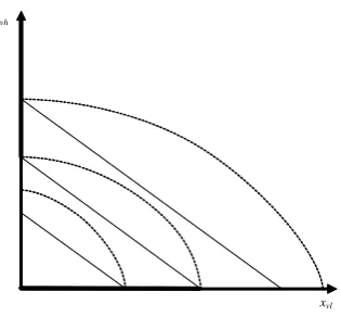
We can thus observe that, for nite prices, each good will eventually upgrade qualitatively, as

illustrated by Figure A1.

To understand the e ect of quality upgrading on the budget shares, we need to be more

speci c on the behaviour of prices. To this aim, we let prices be:

pvi= (v) (qvi) (v)

xvh

xvl

Figure A1:

The quantities consumed of the low- and high-quality goods (xvlandxvh, respectively)

are measured on the axes (horizontal and vertical, respectively). The parallel solid lines represent the intra-good budget constraint for three different levels of incomew

(from left to right, less than, equal to and greater thanw0, respectively). The dotted

lines represent indifference curves. The ticker solid segments on the axes represent the wealth expansion path.

Merella (2010), we normalise the value of the aggregate productivity parameter = 1. Then,

we have:

pvl = (v) ; pvh= (v) (qvh) (v)

and:

xvl =w=[ (v)Q] and xvh= 0 ifw (v) (qvh)

(v)_qvh

qvh 1 _Q

xvl = 0 and xvh =w= h

(v) (qvh) (v) 1Q i

ifw > (v) (qvh)

(v)_qvh

qvh 1 _Q

Finally, denote:

w0= (0) (q0h)

(0)q_0h q_0h 1 _{Q; w}

1 = (1) (q1h)

(1)q_1h q_1h 1 _Q

In line with the Jaimovich and Merella (2010) benchmark model, consider rst the case:

(0) (1) and (0) < (1). In addition, assume (1) _{! 1}. In this case, w0 < w1 =1,

since:

(0) (q0h)

(0)q_0h

q_0h 1 _{(1) (q}

1h)

(1)q_1h q_1h 1 ₌₁

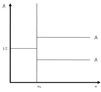
The budget shares are ₀ = ₁ = 1=2 as long as w w0, beyond where 0 rises above 1=2 as

w > w0, as illustrated in Figure A2.

βv

w

Figure A2:

Income is measured on the horizontal axis; the budget shares spent on consumption of the two differentiated goods (βv, withv= 0,1) are measured on the vertical axis.

The solid lines depicting the optimal budget shares (which diverge when incomew

becomes greater thanw0) represent the Engel curves in a budget share form. 1/2

w0

β0

β1

Consider, now, the case: (0) (1) and (0) < (1), assuming (1) is nite. In this case, the budget shares are ₀ = ₁ = 1=2 as long as w w0, beyond where 0 rises (again)

above 1=2 as w > w0. This is eventually followed by an increase in 1 as w > w1. Depending

on the relative value of the high-quality levels, the catching up may be partial (q0h > q1h), full

(q0h =q1h), or 1 may even overtake 0 (q0h < q1h)

Finally, consider the case: (0) > (1) and (0) < (1) < ₁. If (1) is small enough relative to (0), then it may be that:

w0= (0) (q0h)

(0)q_0h

q_0h 1 _{> (1) (q}

1h)

(1)q_1h q_1h 1 _=w

1

Mirroring the previous case, the budget shares are ₀ = ₁ = 1=2 as long as w w1, then 1

rises above 1=2 as w > w1. This is subsequently followed by an increase in 0 asw > w1. Once

again, depending on the relative value of the high-quality levels, the catching up may be partial

D.3 Unit prices at 1-digit level disaggregation

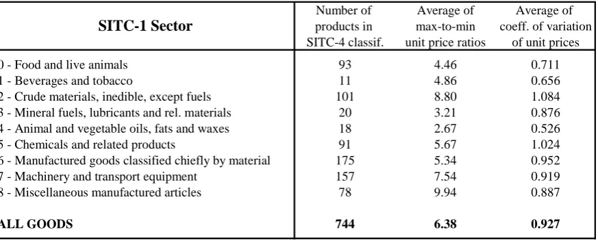
In Table A1 we group all the SITC-4 sectors/goods into their corresponding 1-digit sector.

Therein we report the 1-digit level average values of the interdecile unit price ratios and the

coe cients of variation of unit prices, both calculated at the 4-digit level of disaggregation.

With the exception of sector 2, Table A1 seems to point to the common perception that the

quality ladders of primary goods tend to be shorter than those of manufacturing products (i.e.

sectors 5 to 8).

Table A1:

Number of Average of Average of products in max-to-min coeff. of variation SITC-4 classif. unit price ratios of unit prices

0 - Food and live animals 93 4.46 0.711 1 - Beverages and tobacco 11 4.86 0.656 2 - Crude materials, inedible, except fuels 101 8.80 1.084 3 - Mineral fuels, lubricants and rel. materials 20 3.21 0.876 4 - Animal and vegetable oils, fats and waxes 18 2.67 0.526 5 - Chemicals and related products 91 5.67 1.024 6 - Manufactured goods classified chiefly by material 175 5.34 0.952 7 - Machinery and transport equipment 157 7.54 0.919 8 - Miscellaneous manufactured articles 78 9.94 0.887

ALL GOODS 744 6.38 0.927