A Study on Options Pricing Using GARCH and
Black-Scholes-Merton Model
Zohra Bi
Department of Finance, School of Business, Alliance University, Bangalore, India
E-mail: [email protected]
Abdullah Yousuf
Department of HR, Jain University, Bangalore, India
E-mail: [email protected]
Mihir Dash
Department of Quantitative Methods, School of Business
Alliance University, Bangalore, India
E-mail: [email protected]
Received: Dec. 24, 2013 Accepted: June 17, 2014 Published: June 17, 2014
doi:10.5296/ajfa.v6i1.4830 URL: http://dx.doi.org/10.5296/ajfa.v6i1.4830
Abstract
Options are instruments which have the special property of limiting the downside risk, while not limiting the upside potential, thus their use in hedging. The share of the options market in the Indian capital market has increased to 64% in just over a decade. The trading turnover of options in the FY11 was Rs. 193,95,710 crore, and the trading volume generated by options market was almost two times that of the volume generated in the cash market and futures market put together. So trading and pricing of stock option have occupied an important place in the Indian derivatives market.
problem. The present study applies the GARCH (1, 1) model to estimate the volatility, and applies this estimated volatility to calculate option prices with the help of Black-Scholes-Merton model.
1. Introduction
An option is a derivative financial instrument that specifies a contract between two parties for a future transaction on an asset at a reference price called the strike price. The buyer of the option gains the right, but not the obligation, to engage in that transaction, while the seller incurs the corresponding obligation to fulfill the transaction. In return for assuming the obligation, called writing the option, the originator of the option collects a payment, the premium, from the buyer. So the loss for an option buyer is limited to the premium paid, whereas the loss for an option seller is unlimited. Many options are created in standardized form and traded on an options exchange among the general public, while other over-the-counter options are customized ad hoc to the desires of the buyer, usually by an investment bank. The price of an option derives from the difference between the reference price and the value of the underlying asset plus a premium based on the time remaining until the expiration of the option.
There are two types of options: call options and put options. A call option conveys the right to buy the underlying asset at a specific price, while a put option conveys the right to sell the underlying asset at a specific price. Option contracts have the following specifications: the type (call or put), the quantity and class of the underlying asset, the strike/exercise price (i.e. the price at which the underlying transaction will occur upon exercise of the option), the expiration date (the last date the option can be exercised), and the settlement terms (for instance, whether the writer must deliver the actual asset on exercise, or may simply tender the equivalent cash amount). Also, there are two option styles: European style options can be exercised only on the expiry date, while American style options can be exercised any time before the expiry date.
The Black-Scholes-Merton model (1973) is the most widely-used model of determining option prices. The model expresses the prices of European call and put options on a non-dividend-paying stock in terms of five parameters: the spot price of the underlying stock, the exercise price at which the transaction will be executed, the expiration period after which the option can be exercised, the risk-free rate of return, and the volatility of returns of the underlying stock.
Volatility is a critical factor influencing the option pricing; however, it is an extremely difficult factor to forecast. Hence the crucial problem lies with the accurate estimation of volatility. The estimated volatility can be used to determine future prices of the stock or the stock option, and thus an investor can use arbitrage strategies accordingly to benefit from the model.
2. Literature Review
There is a vast literature on options pricing using the GARCH-Black-Scholes-Merton model. Some of the relevant literature is reviewed in the following.
CNX Nifty 50 index option of India, relative to market price using error metrics, moneyness-maturity-wise. They found that the practitioner Black-Scholes model outperforms the other two models, and reduced the price bias between model and market.
Varma (2002) evaluated the volatility pricing of the index options with the help of the Black-Scholes-Merton option pricing formula and the GARCH (1, 1) model and has found severe mispricing in Indian Index options. He has also established the significant difference in volatility smiles for call and put options. Lehar et al (2002) examined the performance of two extensions of the Black-Scholes-Merton framework, the GARCH and the stochastic volatility option pricing model. They found empirically for FTSE 100 option prices that GARCH dominated over the stochastic volatility and the Black-Scholes-Merton model. However, they found significant errors in the prediction of the market risk from hypothetical derivative positions in all the models.
3. Methodology
The objective of the present study is to analyse systematic mispricing of stock and index options on the NSE using the GARCH model and the Black-Scholes-Merton options pricing model. To analyses the stock options ten companies from ten different sectors, closing stock prices were obtained from the National Stock Exchange1 for the period of 1-May-2012 to 30-Apr-2013 were taken to calculate the volatility using the GARCH(1,1) model for 30-,60-, and 90-day periods. The volatility values thus obtained were used in the Black-Scholes-Merton model to calculate the call and put prices for the stocks.
3.1. GARCH (Generalized Autoregressive Conditional Hetroscedasticity) Model
The Generalized Autoregressive Conditional Heteroscedasticity (GARCH) models were propounded by Engle (1982) and Bollerslev (1986). The distinctive feature of these models is that they recognize that volatilities and correlations are not constant: i.e. volatility clustering and excess kurtosis. The GARCH models are discrete-time models, attempting to track changes in the correlation and volatility over time. The GARCH model is used to estimate volatility for a variety of financial time series: stock returns, interest rates, and foreign exchange rates. GARCH models have been applied in various fields such as asset allocation, risk management, and portfolio management, and option pricing.
The GARCH (p, q) model is formulated as:
,
where p is the order of the GARCH (lagged volatility) terms, and q is the order of the ARCH (lagged squared-error) terms.
average of three different variance forecasts. One is a constant variance that corresponds to the long-run average. The second is the forecast that was made in the previous period. The third is the new information that was not available when the previous forecast was made. This could be viewed as a variance forecast based on one period of information. The weights on these three forecasts determine how fast the variance changes with new information and how fast it reverts to its long-run mean. Volatility and risk both terms are used interchangeably today. If one decides to approach the difficult problem of forecast evaluation, the first consideration is: which volatility is being forecast? For option pricing, portfolio optimization and risk management one needs a forecast of the volatility that governs the underlying price process until some future risk horizon. Future volatility is an extremely difficult thing to forecast because the actual realization of the future process volatility will be influenced by events that happen in the future, e.g. large market movements at any time before the risk horizon. Thus the real problem is that of prediction of volatility. The predicted volatility can be used to determine future prices of the stock or the stock option, and thus an investor can use arbitrage strategies accordingly to benefit from the model.
The GARCH (1, 1) model is represented as , where γ represents the
weight of long run variance; VL represents the long-run variance, α the weight of periodic returns, and β the weight of variance. The parameters α, β and ω are estimated by using the Maximum Likelihood Method, maximizing the log-likelihood function
, subject to the constraint α + β < 1. Once the values of α, β and ω are
obtained, γ = 1 – α – β, and VL is calculated as ω/γ. The annualized volatility is calculated as 251*VL. This volatility is then used to calculate the option prices.
3.2. The Black-Scholes-Merton Model
The Black Scholes-Merton model (1973) is one of the most important concepts in modern financial theory. The BSM model gives the formulae for European call and put options on a non-dividend-paying stock as follows:
Where S represents the spot price of stock, X represents the exercise price of the option, r is
volatility of the stock. In the analysis, for each option, the exercise price was taken at par with the spot price on 1-Jan-2013; the times to expiry considered were 30-, 60-, and 90-days; and the risk-free rate considered was 7.27% p.a. The volatility used was the long-run volatility estimated by the GARCH model.
The market values of the options were compared with the estimated values using the paired-samples Wilcoxon test. The %age difference between the market values and the estimated GARCH-BSM prices were calculated to assess the extent of mispricing. Also, the extent of mispricing for 30-, 60-, and 90-day call and put options were compared using the paired-samples Wilcoxon test.
4. Analysis 4.1 Call Option:
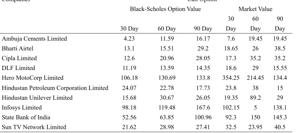
Table 1. Comparison of call option values calculated using Black-Scholes and the Market Option value for 30, 60 & 90 day expiry
Companies Call Option
Black-Scholes Option Value Market Value
30 Day 60 Day 90 Day
30 Day
60 Day
90 Day
Ambuja Cements Limited 4.23 11.59 16.17 7.6 19.45 19.45
Bharti Airtel 13.1 15.51 29.2 18.65 26 38.5
Cipla Limited 12.6 20.96 28.05 17.3 35.2 35.2
DLF Limited 11.19 13.59 14.35 18.6 29 15.55
Hero MotoCorp Limited 106.18 130.69 133.8 354.25 214.45 134.4
Hindustan Petroleum Corporation Limited 24.07 22.78 17.73 23.8 38 15
Hindustan Unilever Limited 15.68 30.67 26.05 19.35 89.2 29
Infosys Limited 98.18 119.48 167.6 102.15 5 138.1
State Bank of India 52.56 63.85 100.96 92.3 150 145.3
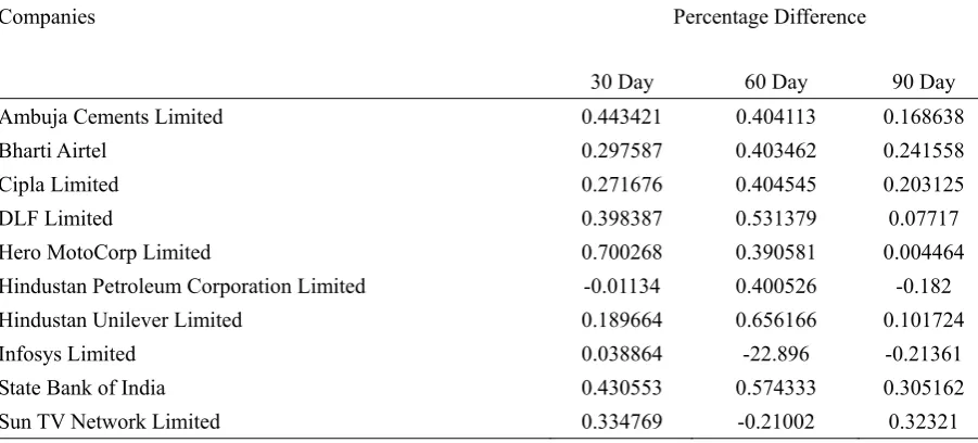
Table 2. Average difference in three different stock call options for different time period of expiry
Companies Percentage Difference
30 Day 60 Day 90 Day
Ambuja Cements Limited 0.443421 0.404113 0.168638
Bharti Airtel 0.297587 0.403462 0.241558
Cipla Limited 0.271676 0.404545 0.203125
DLF Limited 0.398387 0.531379 0.07717
Hero MotoCorp Limited 0.700268 0.390581 0.004464
Hindustan Petroleum Corporation Limited -0.01134 0.400526 -0.182
Hindustan Unilever Limited 0.189664 0.656166 0.101724
Infosys Limited 0.038864 -22.896 -0.21361
State Bank of India 0.430553 0.574333 0.305162
Sun TV Network Limited 0.334769 -0.21002 0.32321
Average difference in call option prices varies based on time effect of 30, 60 & 90 days. There is only a minute difference in the option prices and the above table also shows that the stock call option with 30 days to expiry has a difference which is minimum between the model and market values.
4.2 Put Option:
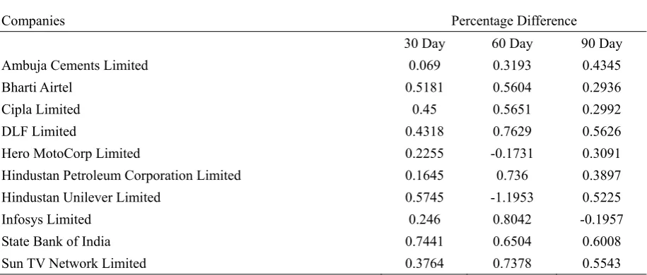
Table 3. Comparison of put option values calculated using Black-Scholes and the Market Option value for 30, 60 & 90 day expiry
Companies Put Option
Black-Scholes Option Value Market Value
30 Day
60
Day 90 Day 30 Day 60 Day 90 Day
Ambuja Cements Limited 16.2 9.7 8.37 17.4 14.25 14.8
Bharti Airtel 8 10.99 17.66 16.6 25 25
Cipla Limited 8.69 8.48 21.27 15.8 19.5 30.35
DLF Limited 9.66 12.21 9.23 17 51.5 21.1
Hero MotoCorp Limited 92.63 72.79 83.57 119.6 62.05 120.95
Hindustan Petroleum Corporation Ltd. 15.75 18.76 11.29 18.85 71.05 18.5
Hindustan Unilever Limited 6.68 13.94 14.11 15.7 6.35 29.55
Infosys Limited 57.91 88.86 113.41 76.8 453.75 94.85
State Bank of India 17.44 44.99 51.38 68.15 128.7 128.7
Sun TV Network Limited 19.3 21.11 17.74 30.95 80.5 39.8
expiry
Companies Percentage Difference
30 Day 60 Day 90 Day
Ambuja Cements Limited 0.069 0.3193 0.4345
Bharti Airtel 0.5181 0.5604 0.2936
Cipla Limited 0.45 0.5651 0.2992
DLF Limited 0.4318 0.7629 0.5626
Hero MotoCorp Limited 0.2255 -0.1731 0.3091
Hindustan Petroleum Corporation Limited 0.1645 0.736 0.3897
Hindustan Unilever Limited 0.5745 -1.1953 0.5225
Infosys Limited 0.246 0.8042 -0.1957
State Bank of India 0.7441 0.6504 0.6008
Sun TV Network Limited 0.3764 0.7378 0.5543
Average difference in put option prices varies based on time effect of 30, 60 & 90 days. There is only a minute difference in the option prices and the above table also shows that the stock call option with 30 days to expiry has a difference which is minimum between the model and market values.
4.3 Paired T-Test
Table 5. SPSS Output of Paired Sample T-Test to compare the model and market prices of thirty day call option price
T-Test
Paired Samples Statistics
Mean N Std. Deviation Std. Error Mean
Pair 1
ThirtydayBSM ThirtydayMV
35.9410 68.6500
10 10
37.304 50 105.602 34
11.796 72 33.394 39
Paired Samples Correlations
N Correlation Sig.
Pair 1
ThirtydayBSM
Paired Differences
95% Confidence
interval of the Difference Pair 1 Thirtyday BSM Thirtyday MV Mean Std. Deviation Std.
Error Mean Lower Upper t df Sig. (2-tailed)
32.709 00 76.511 47 24.195 05 87.442 01 22.024 01 -1.352 9 0.209
Paired sample T-test is done to check whether the numerical difference between the actual and the expected thirty day call option price of stock option which is significant in this case. The SPSS result show that the p value is greater than 0.05. So we can accept the null hypothesis that there is no significant difference between the actual and expected call option prices of stock option.
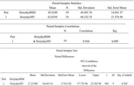
Table 6. SPSS Output of Paired Sample T-Test to compare the model and market prices of sixty day call option price
T-Test
Paired Samples Statistics
Mean N Std. Deviation Std. Error Mean
Pair 1 SixtydayBSM SixtydayMV 45.8100 63.0250 10 10 44.403 36 68.232 35 14.041 57 21.576 96
Paired Samples Correlations
N Correlation Sig.
Pair 1
SixtydayBSM
& SixtydayMV 10 0.564 0.089
Paired Samples Test
Paired Differences
95% Confidence
interval of the Difference Pair 1 SixtydayBSM SixtydayMV
Mean Std.Deviation Std.Error Mean Lower Upper t df Sig. (2-tailed)
17.21500 56.641 61 17.911 65 57.733 96 23.303 96 -961 9 0.362
prices of stock option.
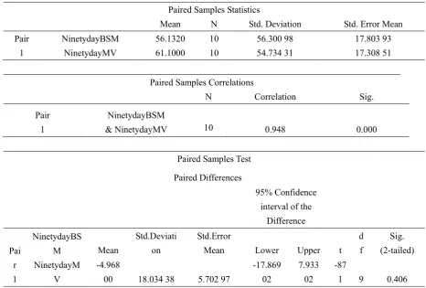
Table 7. SPSS Output of Paired Sample T-Test to compare the model and market prices of ninety day call option price
T-Test
Paired Samples Statistics
Mean N Std. Deviation Std. Error Mean
Pair 1 NinetydayBSM NinetydayMV 56.1320 61.1000 10 10 56.300 98 54.734 31 17.803 93 17.308 51
Paired Samples Correlations
N Correlation Sig.
Pair 1
NinetydayBSM
& NinetydayMV 10 0.948 0.000
Paired Samples Test
Paired Differences
95% Confidence
interval of the Difference Pai r 1 NinetydayBS M NinetydayM V Mean Std.Deviati on Std.Error
Mean Lower Upper t
d f
Sig. (2-tailed) -4.968
00 18.034 38 5.702 97
-17.869 02
7.933 02
-87
1 9 0.406
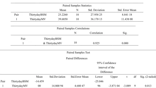
Table 8. SPSS Output of Paired Sample T-Test to compare the model and market prices of thirty day put option price
T-Test
Paired Samples Statistics
Mean N Std. Deviation Std. Error Mean
Pair 1 ThirtydayBSM ThirtydayMV 25.2260 39.6850 10 10 27.958 25 36.170 13 8.841 18 11.438 00
Paired Samples Correlations
N Correlation Sig.
Pair 1
ThirtydayBSM
& ThirtydayMV 10 0.925 0.000
Paired Samples Test
Paired Differences
95% Confidence
interval of the Difference Pair 1 ThirtydayBSM ThirtydayMV
Mean Std.Deviation Std.Error Mean Lower Upper t df Sig. (2-tailed) -14.459
00 14.800 94 4.680 47
-25.046
96 -3.871 04 -3.089 9 0.013
Paired sample T-test is done to check whether the numerical difference between the actual and the expected thirty day put option price of stock option which is significant in this case. The SPSS result shows that the p value is less than 0.05. So we can reject the null hypothesis that there is a significant difference between the actual and expected call option prices of stock option.
Table 9. SPSS Output of Paired Sample T-Test to compare the model and market prices of sixty day put option price
T-Test
Paired Samples Statistics
Mean N Std. Deviation Std. Error Mean
Pair 1 SixtydayBSM SixtydayMV 30.1830 91.2650 10 10 28.937 11 132.681 40 9.150 72 41.957 54
Paired Samples Correlations
N Correlation Sig.
Pair 1
SixtydayBSM
Paired Samples Test
Paired Differences
95% Confidence
interval of the Difference
Pair 1
SixtydayBSM SixtydayMV
Mean Std.Deviation Std.Error Mean Lower Upper t df Sig. (2-tailed) 61.082 00 111.134 79 35.143 91 -140.583 18.419 04 -1.738 9 0.116
Paired sample T-test is done to check whether the numerical difference between the actual and the expected sixty day put option price of stock option which is significant in this case. The SPSS result show that the p value is greater than 0.05. So we can accept the null hypothesis that there is no significant difference between the actual and expected put option prices of stock option.
Table 10. SPSS Output of Paired Sample T-Test to compare the model and market prices of ninety day put option price
T-Test
Paired Samples Statistics
Mean N Std. Deviation Std. Error Mean
Pair 1
NinetydayBSM NinetydayMV
34.8030 52.3600
10 10
36.414 27 44.451 33
11.515 20 14.056 74
Paired Samples Correlations
N Correlation Sig.
Pair 1
NinetydayBSM
& NinetydayMV 10 0.823 0.003
Paired Samples Test
Paired Differences
95% Confidence
interval of the Difference
Pair 1
NinetydayBSM NinetydayMV
Mean Std.Deviation Std.Error Mean Lower Upper t df Sig. (2-tailed) -17.557
00 25.239 35 7.981 38 -35.61214 498 14 -2.200 9 0.55
hypothesis that there is no significant difference between the actual and expected put option prices of stock option.
4.4. MULTIPLE REGRESSIONS
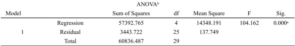
Table 11. SPSS output of Multiple Regression for Stock Call Options:
Regression
Variables Entered/ Removed ᵇ
Model Variables Entered Variables Removed Method
1
Maturity, Stock, Price, Volatility, Strike
Price ᵃ Enter
a. All reserved variables entered b. Dependent Variable: Option Price
Model Summary
Model R R Square Adjusted R square Std. Error of the estimate
1 0.971ᵃ 0.943 0.934 11.73665
a. Predictors: ( Constant), maturity, Stock Price, Volatility, Strike Price
ANOVAᵇ
Model Sum of Squares df Mean Square F Sig.
1
Regression 57392.765 4 14348.191 104.162 0.000ᵃ
Residual 3443.722 25 137.749
Total 60836.487 29
a. Predictors: ( Constant ), maturity, stock Price, Volatility, Strike Price b. Dependent Variable: Option Price
Table 12. SPSS output of Multiple Regression for Stock Put Options:
Regression
Variables Entered/ Removed ᵇ
Model Variables Entered Variables Removed Method
1
Maturity, Stock, Price, Volatility, Strike
Price ᵃ Enter
a. All reserved variables entered b. Dependent Variable: Option Price
Model Summary
Model R R Square Adjusted R square Std. Error of the estimate
1 0.966ᵃ 0.932 0.922 8.5351
a. Predictors: ( Constant), maturity, Stock Price, Volatility, Strike Price
ANOVAᵇ
Model Sum of Squares df Mean Square F Sig.
1
Regression 25142.779 4 14348.191 86.286 0.000ᵃ
Residual 1821.177 25 72.847
Total 26963.957 29
a. Predictors: ( Constant ), maturity, stock Price, Volatility, Strike Price b. Dependent Variable: Option Price
Coefficientsᵃ
Unstandardized
Coefficients
Standardized Coefficients
Model
1
( Constant)
B Std. Error Beta t Sig.
-28.825 5.624 -5.125 0
Stock Price -0.742 0.08 -22.412 -9.277 0
Strike price 0.755 0.079 23.187 9.611 0
Volatility 307.237 54.425 0.436 5.645 0
Maturity -72.704 32.503 -0.163 -2.237 0.034
values are less than 0.05 in all the cases.
5. Discussion
The findings of the study suggest that options are significantly overpriced. However, an interesting possibility suggested by the findings is that this overpricing decreases with expiration period. Also, the findings suggest that put overpricing is significantly higher than call overpricing, as suggested by Dash et al (2012), particularly for longer expiration periods.
The study has several limitations. The sample size used for the analysis is small, and the selected stocks are all large-cap stocks; so that it is not clear whether the results of the study extend to medium- and small-cap stocks. Another difficulty is that of trading volume, which may also affect overpricing, as suggested by Dash et al (2012). Finally, another limitation that may bias the results of the study is the choice of research period; it is not clear whether the results extend to other periods, particularly under high volatility.
There is great scope for applying GARCH option pricing models to examine several other interesting properties of options, including implied volatility, volatility smiles, and the time-variability of options properties (e.g. Greeks).
References
Adesi G.B, Engle. R.F And Mancini.L. (2008). A GARCH option pricing model with filtered historical simulation. Review of financial Studies.
Bakshi.G, C. Cao, & Z. Chen. (1997). Empirical performance of alternative option pricing
models. Journal of Finance, 52, 2003-2049.
http://dx.doi.org/10.1111/j.1540-6261.1997.tb02749.x
Black.F., & M.Scholes. ( 1973). The valuation of option and Corporate Liabilities, Journal of Political Economy, 81,637-654. http://dx.doi.org/10.1086/260062
Christoffwerson.P., & K. Jacobs. (2004). Which GARCH Model for option Valuation.
Journal of Management Science, 50,1204-1221. http://dx.doi.org/10.1287/mnsc.1040.0276
Dash.M, Dagha.J.K., Sharma.P., & Singhal.R. (2012). An application of Garch models in detecting systematic bias in option pricing and determining arbitage in options. Journal of CENTRUM CATHEDRA, 5(1),91-101. http://dx.doi.org/10.7835/jcc-berj-2012-0069
Duan.J. (1995). The GARCH option Pricing Model. Mathematical Finance, 5(1),13-32.
E.Ghysels, & Chernov.M. (2000). A study towards a unified approach to the joint estimation of objective and risk neutral measues for the purpose of option valuation. Journal of Financial Economic, 56,407-458. http://dx.doi.org/10.1016/S0304-405X(00)00046-5
Hao. F., & Yang, H. (2011). Coherent risk measure for derivatives under Black-Scholes economy with regime switching. Journal of Managerial Finance, 37(11),1011-1024.
http://dx.doi.org/10.1108/03074351111167910
application to bond and currency options. Review of financial studies, 6, 327-343.
http://dx.doi.org/10.1093/rfs/6.2.327
Jackwerth, & Buraschi. A. (2001). The Price of a smile: Hedgeing and spanning in option market, 14,495-527.
Jacobs.C., & Christofferson.P. (2004). Which GARCH Model for option valuation. Jounal of management sciences, 50,1204-1221. http://dx.doi.org/10.1287/mnsc.1040.0276
Jacobs.C, Heston, S.L., & Christofferson. P.. a. (2004). A GARCH Option Pricing Model with filtered historical simulation. http://dx.doi.org/10.1287/mnsc.1040.0276
Lehar.A, Scheicher.M., & Schittenkopt.C. (2002). GARCH vs. Stochastic Volatility- Option Pricing and risk management. Journal of Banking & Finance, 26(2/3), 323-346.
http://dx.doi.org/10.1016/S0378-4266(01)00225-4
M.Scholes, & Black.F. (1973). Valuation of options and Corporate liabilities. Journal of political economy, 81,637-654. http://dx.doi.org/10.1086/260062
Nandi.S., & Heston. S. L. (2000). A close form GARCH Option Valuation Model. Review of financial studies, 13(3). http://dx.doi.org/10.1093/rfs/13.3.585
Ross.S.A. Cox. J.C. (1976). The valuation of options for alternative stochastic processes.
Journal of Financial Economics, 3, 145-166.
http://dx.doi.org/10.1016/0304-405X(76)90023-4
Singh.V.P, Ahmed.N, and Pachori.P.(2011). Empirical analysis of GARCH and practitioner Black-Scholes Model for pricing S& P Nifty 50 index options of India. Decision, 38(2),51-67.
Siu.T.K. Tong. H and Yang.H. (2004). On pricing derivatives under GARCH Models: A dynamic Gerber-Shiu's Approach. North American Actuarial journal, 8, 17-31.