The Impact of Financial Leverage on the Cost of Equity

Issues

ISSN: 2146-4138

available at http: www.econjournals.com

International Journal of Economics and Financial Issues, 2019, 9(2), 175-188.

The Impact of Financial Leverage on the Cost of Equity

David Yechiam Aharon

_{*, Yossi Yagil}

1_{Department of Business Administration, Ono Academic College, Kiriat Ono, Israel,} 2_{Department of Business Administration,}

Faculty of Management, University of Haifa, Haifa, Israel. *Email: [email protected]

Received: 12 December 2018 Accepted: 27 February 2019 DOI: https://doi.org/10.32479/ijefi.7554

ABSTRACT

Using a sample of industrial companies traded on the NYSE, this study examines the effect of financial leverage (L) on the cost of equity (K_E). The

goal is to test the theoretical relationship between K_E and L under various types of market imperfections such as taxes and bankruptcy costs, and compare theoretical models incorporating each market imperfection with actual values. All of the empirical results in each model tested point to a

positive relationship between K_E and L regardless of the measures used for the key variables. Specifically, we establish four main findings: (1) The

relationship between K_E and L is positive, (2) R-squared is substantially higher in the risky debt models than in the risk free debt models, (3) The market measures of L tend to generate a higher R-squared than the book measures of L, and (4) The model that is the most accurate representation

of the relationship between the K_E and L incorporates a measure of risky debt. Thus, the findings suggest that risky debt should be employed in the

estimation of K_E, otherwise K_E and the resulting weighted average cost of capital may be biased, leading to incorrect capital budgeting decisions Keywords: Cost of Equity, Financial Leverage, Market Imperfections, Risky Debt

JEL Classifications: G32, G33

1. INTRODUCTION

This paper tests the theoretical relationship between the cost of equity (K_E), and leverage (L) empirically. An initial version of the theoretical relationship between K_E and L was formulated by Modigliani and Miller (MM, 1958) and was later extended to include additional market imperfections such as personal taxes and bankruptcy costs as well as risky debt. Previous studies have examined the relationship between K_E and L empirically, but they did not test the theoretical relationship directly (See for example Dhaliwal et al. 2006). In addition, the theoretical relationship between K_E and L in the presence of risky debt, taxes and bankruptcy costs has not yet been tested directly, nor has the theoretical effect of these variables been compared with their actual counterparts. In this respect, we extend the literature in at least two ways. First, we test the theoretical relationship between K_E and L proposed in the literature directly. Second, we test the degree to which the empirical findings correspond to their theoretical

counterparts. Our findings may help corporate managers and financial analysts estimate K_E when market imperfections are present.

Previous studies have examined how corporate and personal taxes affect a firm’s value and K_E empirically but ignored the possibility of debt default. For example, Mackie-Mason (1990), Dhaliwal et al. (1992), and Graham (1999) investigate the effect of corporate and personal taxes on a firm’s financial leverage and incremental financing decisions. These studies assume that taxes drive the managers’ decisions about capital structure, but they do not provide evidence that the tax implications of debt are reflected in the K_E. Another body of studies focuses on the impact of dividend taxation on the K_E using ex-post realized returns in the case of Dhaliwal et al. (2003) or event studies around changes in the statutory tax rates in the cases of Ayers et al. (2002) and Lang and Shackelford (2000). Dhaliwal et al’s. (2006) study does provide such evidence when they test the K_E expression as a function of

leverage and taxes empirically. They predict that the K_E increases when the firm engages in leveraging and that corporate taxes mitigate this leverage-related risk premium, while the personal tax disadvantage of debt increases this premium. Using estimates for the ex-ante K_E implied by accounting-based valuation models, they generally find evidence consistent with the prediction that corporate tax benefits reduce the leverage-related risk premium demanded by equity investors. However, they point out that the results are sensitiveto the leverage estimates used. To address this issue, in this paper we will conduct robustness tests using eight L estimates based on long-term debt versus total debt, book measures versus market measures, and two computation methods.Note, too, that none of the existing studies includes a comparison between risky debt and risk free debt models in the context of the K_E−L relationship. Therefore, we test this relationship (with the presence of corporate and personal taxes) with and without risky debt. Specifically, we test the K_E−L theoretical relationship (formulated by Yagil, 1982) to determine which model corresponds better with the impact of leverage on K_E-risky debt models or risk free debt models. To mitigate the possible bias of measurement errors and for robustness purposes, we test the K_E−L relationship using several estimates of financial leverage and other key variables such as taxes and bankruptcy costs. Doing so creates an empirical foundation for understanding the impact of managers’ decisions about the capital structure on the K_E. Our empirical tests are divided into two parts. First we determine whether the K_E−L relationship is positive as theory suggests. Then, we test whether the ordinary least squares (OLS) regression coefficients are consistent with the theoretical counterparts for both risky debt and risk free debt models.

The empirical results generally support the theoretical predictions. First, consistent with the extant literature, the K_E is positively associated with financial leverage. All of our tests underscore the positive relationship in both the risk free debt and risky debt models tested. Second, as the results of the risk free debt models imply, the cost of capital decreases with leverage, suggesting that equity holders are compensated with the tax shield created, and the personal taxes associated with debt increase the cost of capital. These results are consistent with Miller’s (1977) study, which argues that individual investors demand a higher return on debt to compensate for the personal tax on interest income. Still, it is worth noting that the results point to a net tax benefit for debt compared to the case of a perfect capital market. Third, the risky debt expressions are a better reflection of the relationship between the K_E and financial leverage than the risk free debt expressions. Most of the results indicate that the regression parameters are more accurate in risky debt models rather than risk free debt assumptions. The R-squared value also supports this point. To summarize, the paper contributes to the recent literature by taking into consideration market imperfections and their impact on the K_E in risk free debt and risky debt models.

The remainder of the paper is organized as follows. Section 2 discusses the scientific background. Section 3 presents the theory and the research hypotheses. Section 4 describes the research sample, data and methods for measuring the variables. Section 5 discusses the results and the robustness tests, while Section 6 summarizes and concludes.

2. SCIENTIFIC BACKGROUND

The empirical literature on the relationship between leverage and K_E is extensive, but inconclusive. While some studies show a positive relationship between K_E and L, others conclude that returns are either insensitive or decline with leverage. Fama and French (1992) and George and Hwang (2007) determine that equity returns are insensitive or even decline with book leverage, but Nielsen (2006) and Penman et al. (2007) find that after controlling for size and book-to-market factors, equity returns are insensitive or fall with market leverage. A large number of studies tested different definitions of expected returns to determine whether there is any empirical relationship. For example, Arditti (1967) finds a negative but statistically insignificant association between leverage and expected equity returns. Using inflation adjusted stock returns for a cross section of all firms including financials without assuming different risk classes, Bhandari (1988) shows that the expected returns increase with leverage. Lang and Shackelford (2000) find evidence of positive abnormal returns when the 1997 Tax Act reduced the tax rate on capital gains from 28% to 20%. Furthermore, they demonstrate that the abnormal returns during the week the 1997 Tax Act became effective decline with leverage. These results suggest that the K_E declines when tax rates on equity income drop, but this effect is smaller for highly leveraged firms. Korteweg (2010) establishes a negative association between stock returns and leverage based purely on changes in the capital structure such as exchange offers. By studying changes in leverage and showing that they are negatively related to current and future returns, Dimitrov and Jain (2008) demonstrate a negative relationship between leveraging and stock returns. Dhaliwal et al. (2006) examine the associations among leverage, corporate and investor level taxes, and the firm’s implied K_E. Their results suggest that the equity risk premium associated with leverage declines with the corporate tax benefits from debt. They find some evidence that the equity risk premium from leverage increases with the personal tax penalty associated with debt. Dhaliwal et al. (2007) demonstrate that the implied K_E decreased after the 2003 Tax Act reduced the tax rate on dividends from 38.6% to 15% and the tax rate on capital gains from 20% to 15%. George and Hwang (2007) find a negative relationship between returns and leverage. They also argue that firms that are affected more adversely by financial distress engage in lower leverage. Penman et al. (2007) investigate the book-to-price effect in expected stock returns and its relation to leverage, demonstrating that the leverage component is negatively related to ex-ante stock returns. Gomes and Schmid (2010) and Obreja (2013) explore returns using dynamic models in which capital structure and investment decisions interact, thus violating the assumption of MM about the separation between financing and investment decisions. Obreja’s (2013) model studies the interaction between book-to-market and leverage. After calibration, the model is able to generate samples that replicate the empirical evidence provided by Bhandari (1988) and Fama and French (1992). George and Hwang (2010) argue that leverage may be negatively correlated with future returns because highly leveraged firms are less exposed to systematic distress risk. This could be true because firms facing high distress costs endogenously choose low financial leverage.

However, a key factor missing in these studies is risky debt, which can be associated with bankruptcy costs. Despite the extensive empirical literature, there is no study that examines the effect of risky debt associated with bankruptcy costs on returns in a direct manner provided here. Furthermore, there are no studies comparing risky debt results with corresponding situations that assume risk free debt. Thus, we test the K_E−L relationship for the case of risky debt and bankruptcy costs as well as when market imperfections such as corporate and personal taxes exist.

3. THEORY AND HYPOTHESES

Following MM, Yagil (1982) derived the general theoretical expression that links the K_E to the corporate and personal tax rates, assuming risky debt associated with bankruptcy costs. Eq. (1) expresses this relationship:

K_E = K_U+[K_U(1−Ψ]−R(1−T_C)(1−T_E)]L, (1)

Where K_E is the K_E, K_U is the return required by equity holders for the unleveraged firm, Ψ is (1−q−T), which is the factor that includes the bankruptcy factor (q) as a percentage of the firm’s debt, the tax ratio (T) given by (1−T_C)(1−T_E)/(1−T_D), T_C is the corporate tax rate, T_E is the tax rate applicable to equity holders and T_D is the tax rate for debt holders, R is the cost of risky debt, and L is the financial leverage ratio of debt to equity (D/E) where D and E are the values of the debt and equity, respectively.

In the absence of taxes and risk free debt, Ψ=0 and Equation (1) reduces down to:

K_E=K_U+[(K_U–r)L] (2)

Which is equivalent to MM Proposition II for the K_E in the absence of taxes. Eq. (2) states that K_E is equal to the K_E for the unleveraged firm plus a premium expressed as the product of the leverage ratio (L) and the spread between K_U and the cost of debt, which in this case, is simply the risk free rate of interest. If corporate taxes are the only market imperfection and debt is risk free, Ψ reduces down to T_C, and Equation (2) becomes:

K_E=K_U+(1−T_C)(K_U–r)L (3)

This equation is equivalent to MM’S tax case expression. Eq. (3) indicates that the risk premium is lower than its value in Equation (2), due to the tax deductibility of debt financing.

If personal taxes are a factor in addition to corporate taxes, and debt is still risk free, then q=0, and Ψ is simply (1−T). Thus, Equation (1) will be reformulated as Equation (4):

K_E=K_U+T[K_U−r(1−T_D)]L (4)

In theory, as the tax rate on interest income increases relative to the tax rate on equity income, bondholders demand higher relative pretax returns to leave them equally well off on an after-tax basis. The resulting higher interest cost reduces the tax benefits of debt accruing to equity holders. As a result, the equity risk premium

from leverage should increase in the personal tax penalty on interest income and decrease from the effect of the corporate tax shield.

Equations. (2-4) describe the return that equity holders require when relaxing the assumption of risk free debt. If debt is considered risky and corporate and personal taxes exist, then Ψ simply equals (−q), and Equation (1) is reformulated by Equation (5):

K_E=K_U+[K_U(1+q)–R]L (5)

If personal taxes do not exist, then Ψ=[1−(1−T_C)−q], which is simply (T_C−q), and Equation (1) will be phrased as Equation (6):

K_E=K_U+[K_U(1−T_C+q)–R(1−T_C)]L (6)

It is worth noting that Equation (5) and Equation (6) differ from their corresponding risk free formulations only in the addition of the bankruptcy costs factor (q) in the coefficient of the financial leverage ratio of the firm. Since the value of q is surely a positive term, it indicates the extra penalty in the K_E as the risk of default increases. Note too that if only debt is considered risky, and there are no taxes or bankruptcy costs, then Equation (1) is simply the following Equation (7):

K_E=K_U+[K_U–R]L (7)

According to Equation (7), K_E is the K_E which is the required return by equity holders for the unleveraged firm plus a premium related to the product of the financial leverage ratio (L) and the spread between the return required for the unleveraged firm (K_U) and the cost of the risky debt (R).

To summarize, we present seven different formulations to describe the relationship between the K_E and financial leverage. Equations 2-4 deal with the risk free debt models. Equation (2) describes the perfect capital market case, Equation (3) assumes corporate taxes only, and Equation (4) takes into account both corporate and personal taxes. Similarly, for the risky debt models, Equation (1) is the formulation for the K_E when corporate and personal tax rates exist, and debt is risky and associated with bankruptcy costs. Equation (5) deals with the situation where only corporate taxes exist. Equation (6) considers both corporate and personal taxes. Finally, Equation (7) describes the perfect capital market case but debt is risky.

We test the relationship between K_E and L using these regression models. The first three models represent the case of risk free debt, which we call henceforth “Case A.” The other four models represent the case of risky debt, which we call henceforth “Case B.” Model (1) (both equations 1a and 1b below) is for the case of perfect capital markets. Model (2) (both 2a and 2b) is for the case where corporate taxes are the only type of market imperfection. Model (3) (both 3a and 3b) is for the case of both corporate and personal taxes. Model (4b) incorporates bankruptcy costs as well. The equations governing these models appear below:

Case A: Risk free debt models:

K_E=K_U+[(K_U–r)(1−T_C)L] (2a)

K_E=K_U+T[K_U−r(1−T_D)]L (3a)

Case B: Risky debt models:

K_E=K_U+[(K_U–R)L] (1b)

K_E=K_U+[(K_U–R)(1−T_C)L] (2b)

K_E=K_U+T[K_U−R(1−T_D)]L (3b)

K_E=K_U+[K_U(1−Ψ)−R(1−T_C)(1−T_E)]L (4b)

Starting with the first model, the direct estimation of Equation (1a) where market frictions do not exist and debt is risk free is as follows:

K_E=γ₀+γ₁[L] (11)

In this case, the dependent variable is the K_E, which we estimate using the familiar capital asset pricing model (CAPM), and the term in the squared brackets is the independent variable, which is simply the financial leverage of the firm.

The null hypothesis from regressing L directly versus K_E is that the intercept of this equation model γ₀ represents K_U.If γ₀ truly represents K_U, the observed γ₀ parameter will not differ statistically from(K_E+rL)/(1+L), which is the K_U derived by unlevering Equation (1a). Similarly, if Equation (1a) holds true, γ₁ should be equal to the value of (K_U–r). To test whether γ₀ and γ₁ correspond to their theoretical counterparts, we use the mean value of K_U derived for each firm, the risk free rate (r) and the financial leverage (L).

Accordingly, if corporate tax is the only market friction, then the direct estimation model is:

K_E=γ₀+γ₁[(1−T_C)L] (12)

The term in the squared brackets is the explanatory variable used, and K_E is again the dependent variable. According to this specification, γ₀ should be equal to K_U, which is estimated as the mean value across of all firms by K_U= (K_E+r(1−T_C)L)/(1+(1−T_C)L), and γ₁ should be equal to the value of (K_U–r). Theory suggests that due to corporate taxes, the equity risk premium from leverage here is smaller by a factor of one minus the corporate tax rate. In other words, the tax benefit from debt offsets the leverage-related risk premium demanded by equity holders. Thus, comparing the results of the perfect capital market with the case of corporate taxes only should yield a slope that is closer to (K_U–r) in the last case relative to the perfect capital market case. Next, if personal taxes also exist, the direct estimated regression equation is:

K_E=γ₀+γ₁[TL] (13)

In this case K_U is estimated by [(K_E+TLr(1−T_D)]/(1+TL). Thus, if Equation (3a) holds true [tested by Equation (13) above], γ₀ should be equal to the K_U derived above and γ₁ to the value of [K_U

−r(1−T_D)]. Note that the effect of leverage on the K_E is positive as long as the after-tax return on equity is greater than the after-tax return on debt. According to the theory, the firm’s K_E increases with leverage, decreases with the firm’s tax benefit from debt, and finally, increases withthe personal tax penalty associated with debt.

In cases where the debt is considered risky and taxes do not exist, the estimated regression of Equation (1b) will be as follows:

K_E=γ₀+γ₁[(K_U–R)L] (14)

Note that the only difference now is that R is the cost of debt, which is estimated exogenously by applying the CAPM according to the beta of debt (β_D). In this case γ₀ should be equal to K_U and γ₁ should be equal to 1. In cases where the debt is considered risky and corporate taxes do exist, the estimated regression of Equation (2b) will be as follows:

K_E=γ₀+γ₁[(K_U–R)(1−T_C)L] (15)

Where the null hypothesis (H0) is that γ₀=K_U and γ₁=1. When personal taxes are introduced, the direct estimation of Equation (3b) will be as follows:

K_E=γ₀+γ₁T[K_U−R(1−T_D)]L (16)

Accordingly, by the null hypothesis, γ₀=K_U and γ₁=1. In other words, if Equation (3b) [tested by Equation (16) above] represents the true relationship between the K_E and financial leverage when debt is risky and corporate and personal taxes exist, the observed γ₀ should be no different from K_U. In this situation, K_U is the mean value of the required return by equity holders for a pure equity firm, and γ₁ should be no different from 1, because theoretically, all market imperfections are included except bankruptcy costs. Finally, we test the last equation, Equation (4b), which includes corporate and personal taxes, and risky debt associated with bankruptcy costs. We use the following regression equation to estimate Equation (4b):

K_E=γ₀+γ₁{[K_U[(1−Ψ]−R(1−T_C)(1−T_E)]L} (17)

Where the term in the curly brackets is the explanatory variable, where the null hypothesis is γ₀=K_U and γ₁=1.

To summarize, the empirical methodology involves testing seven different models. The comparison of the results may possibly allow us to identify which models (risk free or risky debt) correspond to the theoretical K_E–L relationship. One of the important reasons for making this determination is that K_E is one of the components of the weighted average cost of capital (WACC) that is used in capital budgeting decisions. Using inappropriate models might lead to incorrect decisions based on a bias in the estimation of the K_E and the net present value of the firm’s projects.

4. DATA AND VARIABLE MEASUREMENT

4.1. Data

the adjusted stock prices. For each firm in the sample, we gathered the following accounting data: The total debt, long term debt, total equity, pretax income and total taxes paid, total dividend paid and number of shares of preferred stock, and also the historical stock returns in the preceding 5 years to each sample year. Due to data availability, our sample ends in 2007 since The University of Haifa’s subscription to COMPUSTAT ended in 2008. Thus, we could not gather data after 2007. Given that we needed data from five normal years before our start date, we begin with the period of 2003 since the preceding years were associated with the high-tech bubble years that resulted in abnormal returns.

Testing the various theoretical models outlined above requires a reference to the risk class issue. Theory states that K_U should be identical across all firms in the same risk class. Consequently, an empirical problem that can arise is that K_U is supposed to be constant in the defined risk class, but practically it may vary across the companies in the same risk class. Taken to the extreme, K_U may practically even vary from one company to another. The empirical tradeoff involved then, is between selecting a very small sample in order to maintain a homogenous risk class on one hand, and the low statistical reliability that may be associated with a relatively small sample. Given this tradeoff, we selected our sample to consist of the Industrial sector according to the GICS definition of COMPUSTAT and, at the same time, is sufficiently large for obtaining statistically reliable results. Furthermore, in order to reduce the “survival bias” discussed in the literature, our sample in the various years contains precisely the same set of companies (which naturally reduced the size of our initial sample). In addition,

to minimize the potential measurement errors caused, among other things, by our relatively broad risk class assumption, we employed various sensitivity analyses and robustness tests discussed later in this study. The initial sample consisted of all 306 firms from the Industrial sector covered by COMPUSTAT. We then required a complete data (as detailed above) for each of the companies in the sample and for each of the sample years. This additional screening procedure reduced our sample down to 182 firms.

4.2. Variable Measurement

We investigate the relationship between K_E and L will be tested here by employing an OLS regression analysis. This relationship will be investigated for different types of market imperfections such as corporate taxes, personal taxes and bankruptcy costs. The general analysis will use the following variables: The K_E, the financial leverage (L), the values of debt (D) and equity (E), tax rates, both corporate (T_C) and personal (T), and the bankruptcy costs factor (BC). We use several estimates of the financial leverage and tax variables to test the robustness of the results and to mitigate the potential problem of measurement errors. In the next sub sections we describe in detail the estimation procedure for each of the above key variables.

4.3. KE

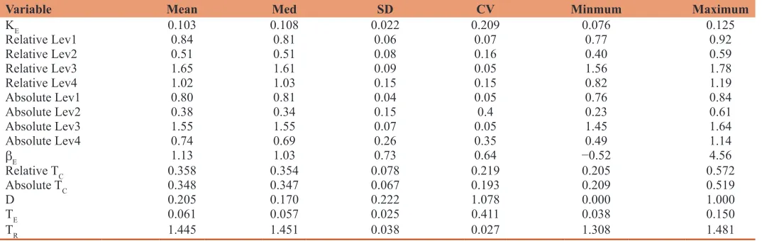
Table 1 reports the descriptive statistics for the two key variables in this study: The K_E and the financial leverage (L). Following the familiar procedure in the literature, we use the CAPM for measuring the K_E to each firm in the sample. Specifically, we measure K_E of each firm using K_E=r+β_E(E_m−r). In other words, the

Table 1: Descriptive statistics of the corporate variables ($M)

Variable Mean Med SD CV Minmum Maximum

K_E 0.103 0.108 0.022 0.209 0.076 0.125

Relative Lev1 0.84 0.81 0.06 0.07 0.77 0.92

Relative Lev2 0.51 0.51 0.08 0.16 0.40 0.59

Relative Lev3 1.65 1.61 0.09 0.05 1.56 1.78

Relative Lev4 1.02 1.03 0.15 0.15 0.82 1.19

Absolute Lev1 0.80 0.81 0.04 0.05 0.76 0.84

Absolute Lev2 0.38 0.34 0.15 0.4 0.23 0.61

Absolute Lev3 1.55 1.55 0.07 0.05 1.45 1.64

Absolute Lev4 0.74 0.69 0.26 0.35 0.49 1.14

β_E 1.13 1.03 0.73 0.64 −0.52 4.56

Relative T_C 0.358 0.354 0.078 0.219 0.205 0.572

Absolute T_C 0.348 0.347 0.067 0.193 0.209 0.519

D 0.205 0.170 0.222 1.078 0.000 1.000

T_E 0.061 0.057 0.025 0.411 0.038 0.150

T_R 1.445 1.451 0.038 0.027 1.308 1.481

Table 1 reports the descriptive sample statistics. All financial statement data is gathered from the COMPUSTAT database. The values reported are measured in $millions except for common shares outstanding. The reported statistics are the Mean, Median (Med), Standard Deviation (SD), coefficient of variation (CV), Minimum (Min) and Maximum (Max). Lev1 is the ratio of LTD/Equity_BV, Lev2 is the ratio of LTD/Equity_MV, Lev3 is the ratio of (LTD+CL/Equity_BV) and Lev4 is the ratio of (LTD+CL/Equity_MV), where Lev denotes the financial leverage, LTD is long-term debt in book value, equity is the total value of common equity, CL is current liabilities and the subscripts BV and MV stand for book and market values, respectively. The estimate of the financial leverage for each year is based on the mean value over the preceding five years. Two such estimates have been constructed--Relative and Absolute. The relative Lev estimate for a given year is the mean value of the Lev variable across the preceding five years, while the Absolute Lev is given as the 5-year mean value of the “debt” numerator divided by the 5-year mean value of the “equity” denominator. Using the CAPM, we estimate K_E for each year where K_E=r+β(Em−r), r is the 1-year Treasury Constant Maturity Rate as a proxy for the risk free rate of interest, which equals 1.2%. 1.9% and 3.6% for 2003, 2004 and 2005, and 4.9%, 4.5% for 2006, 2007, respectively, β is the systematic equity risk derived from historical 60 monthly returns for both the stock and the market index (NYSE), and (Em−r) is the market risk premium estimate which is 6% here based on the surveys of Fernandez, Aguirreamalloa and Linares (2013). The Relative TC estimate for a given year is the mean value of the TC variable across the preceding five years, while the

Absolute T_C is given by the 5-year mean value of the firm’s total tax expense divided by the 5-year mean value of the firm’s taxable income. The table also reports the payout ratio (d), the personal tax rate (TE) and the taxes ratio [(TR); TR=(1−TE)/(1−TD)]. TE is the tax rate applicable to equity holders, and TD is the tax rate applicable to debt holders. TD is the highest

statutory tax rate on interest income, which is 39.6% for 1998 through 2000, 38.6% for 2001 through 2002 and 35% thereafter. We estimate T_E as a weighted-average tax rate on dividend and capital gains income using the following term: TE=[d Td+(1−d)αTcg], where d is the proportion of the net income distribution paid out in dividends, and (1−d) is the retention ratio.

Following the procedure devised by Dhaliwal, Heitzman and Li (2006), we winsorize d at zero and one. T_d is the personal tax rate on dividend income, set equal to the values of T_D for years prior to 2003, and 15% thereafter. Tcg is set equal to the top statutory tax rate on long-term capital gains income, which equals 20% for 1998 through 2002 and 15% thereafter. α is

K_E for a particular stock is simply the risk free rate of return (r) plus the product of the market premium risk (E_m) and equity systematic risk (β_E). Accordingly, we estimate the β_E by regressing the stock’s rate of return against the market index’s rate of return, in this case, the NYSE composite index. We use 60 monthly returns for both the stock index and the market index. Given that the sample consists of NYSE stocks, the market index employed here is the NYSE Composite index. Table 1 reports the descriptive statistics of the β_E estimate for each year. We measure r as the 1-year Treasury Constant Maturity Rate published by the Board of Governors of the Federal Reserve System. Accordingly, the risk free rate of return in each year is 1.2%. 1.9% and 3.6% for 2003, 2004 and 2005, and 4.9%, 4.5% for 2006, 2007, respectively.

We then construct the risk premium estimate based on surveys conducted by Fernandez et al. (2013), who report that the risk premium for the U.S capital market was 6.3%, 6%, 6%, for 2008, 2009, 2010, 5.5% in 2011 and 2012, and 5.7% in 2013. Accordingly, our estimate for the risk premium is 6%. To test the robustness of our findings, we also used 5% and 7%, and obtained similar results regardless of the estimated E_m.

4.4. Financial Leverage

The literature suggests a long list of financial leverage variables that are book or market measures. Appendix 1 presents a summary of the financial leverage estimates in recent studies. While the market estimation of equity is available, it is difficult to assess the debt component due to the problem of gathering the historical market value of debt and other statistical problems such as stationary in bond prices. As a result, most studies use book measures for the financial leverage or a hybrid financial leverage ratio that combines market equity estimations with the book value of debt. Many studies consider the latter a market measure. In addition, the literature refers to various types of debt such as short-term, long-term and total debt. Denis and McKeon (2012) use the total debt over total debt plus the market value of equity. Giroud et al. (2012) define the market measure of financial leverage as the ratio of the book value of total debt to the book value of assets. George and Hwang (2010) calculate the ratio of the book value of long-term debt to the book value of assets, while Brav (2009) uses the ratio of short-term debt plus long-term debt to total assets. Based on recent studies we create four estimates of financial leverage: (1) Lev1=LTD/Equity_BV, (2) Lev2=LTD/ Equity_MV, (3) Lev3=(LTD+CL)/Equity_BV, (4) Lev4=(LTD+CL)/ Equity_MV, where Lev denotes financial leverage, LTD is long-term debt, Equity is the value of common equity, CL is current liabilities, and the subscripts BV and MV stand for book and market values, respectively. Equity_MV includes the common equity in MV calculated as the product of the number of common shares outstanding and the mean value of the 12 monthly closing stock prices. We also used the leverage ratios that include preferred stock, and the results remained very similar. The estimate of financial leverage (Lev) for each year is based on the mean value of the preceding 5 years. We also create two such estimates--relative and absolute. The Relative Lev estimate for a given year is the mean value of the Lev variable across the preceding 5 years, while the Absolute Lev is calculated as the 5-year mean value of the “debt” numerator divided by the 5-year mean value of the “equity”

denominator. To summarize, we use eight different versions of the financial leverage ratio in the empirical analysis – four for each of the two calculation methods—relative and absolute. Table 1 presents a summary of the statistics for the various leverage estimates used in this study.

4.5. Corporate and Personal Taxes

Following Arena and Roper (2010), and Dyreng et al. (2010), we use the total tax expense divided by pretax income as the corporate tax rate variable (T_C). We estimate T_C for each firm in each year based on the mean value of the preceding 5 years. Accordingly, we again construct two estimates - relative and absolute - to test the sensitivity of the results. The Relative T_C estimate for a given year is the mean value of the T_C variable across the preceding 5 years. The Absolute T_C is given by the 5-year mean value of the firm’s total tax expense divided by the 5-year mean value of the firm’s taxable income. The tax ratio (T_R) is defined here as: T_R=[(1−T_E)/ (1−T_D)], where T_D is the tax rate for debt holders, and T_E is the tax rate applicable to equity holders. T_E is the weighted-average tax rate on dividends and capital gains income. In other words, it is the tax rate on dividends (T_d) and capital gains (T_cg) income expressed as: T_E=[d T_d+(1−d)·α·T_cg], where d is the dividendpayout ratio computed as the most years’ dividend divided by the mean value of the net income over the prior 3 years. Accordingly, (1−d) is the earnings rate. Following the procedure devised by Dhaliwal et al. (2006) we winsorize d at zero and one. T_d is the personal tax rate on dividend income, set equal to the values of T_D for the years prior to 2003, and 15% thereafter. T_cg is set equal to the top statutory tax rate on long-term capital gains income, which equals 20% for 1998 through 2002, and 15% thereafter. α is the benefit of capital gains deferral. Following Van Binsbergen et al. (2010), Graham (1999), and Dhaliwal et al. (2006), we assume that α=0.25. Following Dhaliwal et al. (2006), T_D is measured as the highest statutory tax rate on interest income, which is 39.6% for 1998 through 2000, 38.6% for 2001 through 2002, and 35% thereafter. The final results are similar to those of Dhaliwal et al. (2006), while the relative and absolute computation methods also yield very similar estimates.

4.6. The Required Return on Debt

As with the K_E, we also use the CAPM to estimate the required return on debt (R) with the following equation: R= r+β_D(E_m−r), where R is the required return on the firm’s debt, β_D is the debt beta coefficient, (E_m−r) is the market risk premium and r is the 1-year U.S Treasury Constant Maturity Rate as a proxy for the risk free rate of interest. The market premium (E_m−r) estimate is based on the surveys of Fernandez et al. (2013). As stated earlier in sub section 4.3 using other estimates of 5% and 7% obtained similar results.

potential measurement errors, we employ below a range of mean bond betas of 0.1, 0.2 and 0.3 that may appear consistent with the mean bond beta values reported in the literature, and which very likely may contain the true unobservable mean bond betas. Each mean value is then adjusted separately for each firm to reflect the individual bond beta by incorporating the deviation of the specific company’s financial leverage from the entire sample financial leverage. Consider for example the following parameter values: the mean and standard deviation of β_D for the entire sample are 0.3 and 0.063 (based on Bloomberg ETF sample), the mean and standard deviation values for the financial leverage of the entire sample of 1.5 and 0.5, respectively, and the specific company’s financial leverage is 2.5. The estimate for the specific company’s β_D then will be given as follows: β_D=0.3+20.063=0.426, where the Z score of 2 is given by: (2.5−1.5)/0.5=2.

Note also, that for compatibility purposes we estimated debt betas using the same market index – the NYSE composite index. With regard to the equity betas, we followed the practice in the empirical literature and employed an all-equity index for estimating the stock betas. Given this practice, using the same index for bonds as well may result in a lower bias than using an alternative index such as an all-debt index or a debt-and-equity index Weinstein (1981) also employed the NYSE index for estimating bond betas); It seems that it is not an uncommon practice

4.7. Bankruptcy Costs

Over the years since the first publication of MM study, researchers have tried to determine the association between market frictions and capital structure. One of the potential frictions that affect the K_E is expected bankruptcy costs. The literature includes a variety of studies in the context of bankruptcy costs, but we focus on the most recent ones. Estimating such costs has proven difficult and yielded mixed results. For example, in a study of companies entering Chapter 7 or Chapter 11 proceedings, Bris et al. (2006) find that bankruptcy costs range from 2% to 20% of a firm’s assets but advise caution when using these results. They argue that their measures are sensitive to the procedure, particularly to the denominator (how the assets are measured). More specifically, they advise theorists not to claim either uniformly low or uniformly high bankruptcy costs, but rather to recognize that bankruptcy costs are modest in some firms and large in other firms. Garlappi and Yan (2011) provide a measure of expected default probability (EDF, henceforth - p). A firm’s p measure represents an assessment of the likelihood of default for that firm within a year. They report an average p measure of 3.30%. They also state that 75% of firms have a default probability of <3.5%, and about 5% of firms have a p score of 20%. Finally, Hortaçsu et al. (2013) present a mechanism through which a firm’s decisions about its financial structure create indirect costs of financial distress in the auto market. Using wholesale auction prices, credit default swap spreads, and data for used cars sold, they find that a 1,000-basis-point movement in credit default swap spreads causes a price reduction of $68 - about 0.5% of the average sales price in their sample.

Warner (1977) estimates the direct bankruptcy costs of 11 US railroad companies that were in bankruptcy proceedings from 1933 to 1955. He finds that these costs averaged 1% of the market

value of the firm 7 years before entering into Chapter 11 and rose to 4% 1 year prior to bankruptcy. However, Warner notes that his results should be interpreted cautiously because they are based on a narrowly defined bankruptcy cost definition. In addition, his small sample of railroad bankruptcies is not necessarily indicative of the population of firms. Weiss (1990) conducts a study on 37 industrial firms between 1979 and 1986. He finds that on average, the direct costs are 3.1% of the book value of the debt and market value of the firm’s equity. Miller (1977) argues that the direct cumulative bankruptcy costs average only 5.3% of the value of the firm and 1.7% for the largest firms. Miller also suggests that the total loss of the market value 84 months prior to the bankruptcy date equals 1.3% of the firm’s value. Altman (1984) estimates the total bankruptcy costs (both direct and indirect) as 16.7% of a firm’s value in the year in which the firm becomes insolvent, 11.2% of the firm’s value 1 year prior to the bankruptcy, 11.7% of the firm’s value 2 years prior to the bankruptcy and 12.4% of the firm’s value 3 years prior to the bankruptcy. He also argues that indirect bankruptcy costs are not limited to firms that actually fail. Firms that have a high probability of bankruptcy, whether they eventually fail or not, can still incur these costs. Andrade and Kaplan (1998) point out that many previous studies that examined the indirect costs of financial distress fail to distinguish financial distress from economic distress. By examining a sample of 31 highly leveraged transactions, their results show that the indirect costs of financial distress are 10–23% of a firm’s value.

To create a reliable estimate of the bankruptcy costs factor (q), we use a set of four alternative measures--3%, 7%, 11%, and 15%--to proxy for the true value of bankruptcy costs. Since a higher level of financial leverage is associated with a greater potential for bankruptcy, we adjust the coefficient of each firm’s specific expected bankruptcy costs according to the relative Z score derived from its estimated degree of financial leverage. Note too that q=C/D, where C is the expected value of the bankruptcy costs, and D is the value of the debt. In determining this set we already took into account that q is in terms of the debt rather than the total value of the firm in the empirical studies referred to at the beginning of the current section.

5. EMPIRICAL FINDINGS

5.1. Descriptive Statistics

Similarly, the median value of the relative and absolute Lev₁ is 0.81, while the median value of the corresponding market measures is 0.51 and 0.34. Similar results were found for Lev₃ and Lev_4, which consider the total debt of the firm. The bottom of Table 1 reports the descriptive statistics for the tax variables including corporate and personal taxes. It can be noticed that the relative and absolute measures for the corporate taxes yield similar results. Overall, the mean value across the sample years is 0.358 and 0.348 for the relative and absolute measures. Using the median values yield similar results. Note too, that in the context of personal taxes, our results are similar to those of Dhaliwal et al. (2006). The mean

value of the tax ratio (T_R) in their study for 2003 and 2004 (their study ends in 2004) is 1.450, while in our study it equals 1.440 and 1.441. Overall, the mean value across the sample years is 1.445. Finally, with accordance to Dhaliwal et al. (2006) study the majority of the sample firms pay dividends, because the median payout ratio (d) is positive in each sample year.

5.2. Regression Results

Table 2 presents the regression results for testing Equation s. (1a)- (4b), starting with the perfect capital market in the risk free debt model, and ending with the case including taxes and

Table 2: Regression results

Lev4(Mv) Abs Mean Median SD Minimum Maximum

Case A: Risk free debt models

Model (1a) K_E=K_U+(K_U−r)[L], K_E=γ₀+γ₁[L] Intercept 0.076 0.078 0.022 0.050 0.100

Slope 0.018 0.019 0.005 0.011 0.023

R2 _{0.195 0.217 0.084 0.077 0.278}

Slope Sig 0.000 0.000 0.000 0.000 0.000 Model (2a) K_E=K_U+(K_U−r)[(1−Tc) L], K_E=γ₀+γ₁[(1−Tc) L] Intercept 0.085 0.087 0.024 0.057 0.110

Slope 0.034 0.035 0.008 0.022 0.043

R2 _{0.185 0.201 0.088 0.080 0.276}

Slope Sig 0.000 0.000 0.000 0.000 0.000

Model (3a) K_E=K_U+[K_U−r(1−T_D)][TL], KE=γ₀+γ₁[TL] Intercept 0.085 0.087 0.024 0.057 0.110

Slope 0.023 0.024 0.005 0.015 0.030

R2 _{0.189 0.205 0.089 0.085 0.281}

Slope Sig 0.000 0.000 0.000 0.000 0.000

Case B: Risky debt models

Model (1b) K_E=K_U+[(K_U−R) L], K_E=γ₀+γ₁[(KU−R) L] Intercept 0.067 0.070 0.025 0.036 0.093

Slope 1.027 1.017 0.067 0.940 1.098

R2 _{0.417 0.413 0.126 0.282 0.587}

Slope Sig 0.000 0.000 0.000 0.000 0.000 Model (2b) K_E=K_U+(K_U−R)(1−Tc) L, K_E=γ₀+γ₁[(K_U−R)(1−Tc) L] Intercept 0.064 0.067 0.025 0.032 0.089

Slope 1.145 1.122 0.130 1.017 1.334

R2 _{0.547 0.500 0.153 0.420 0.718}

Slope Sig 0.000 0.000 0.000 0.000 0.000 Model (3b) K_E=K_U+T[(K_U−R(1−T_D)]L, K_E=γ₀+γ₁{T[(K_U−R(1−T_D)]L} Intercept 0.061 0.064 0.024 0.031 0.086

Slope 1.054 1.033 0.119 0.936 1.227

R2 _{0.547 0.500 0.153 0.420 0.718}

Slope Sig 0.000 0.000 0.000 0.000 0.000 Model (4b) K_E=K_U+[K_U(1−Ψ)−R(1−T_C)(1−T_E)]L,

K_E=γ₀+γ₁[K_U(1−Ψ)−R(1−T_C)(1−T_E)]L Intercept_Slope 0.063_1.475 0.064_1.465 0.021_0.153 0.040_1.290 0.085_1.690

R2 _{0.663 0.664 0.039 0.605 0.706}

Slope Sig 0.000 0.000 0.000 0.000 0.000 Table 2 presents the regression results of: Model (1a): KE=KU+KU[L] using the estimated regression equation given by: KE=γ0+γ1[L]. Model (2a): KE=KU+KU[(1−TC) L] using the estimated regression equation given by: KE=γ0+γ1[[(1−TC) L], Model (3a): KE=KU+KU[TL] using the estimated regression equation given by :KE=γ0+γ1[TL], Model (1b):

KE=K_U+[(K_U−KD) L] using the estimated regression equation given by: KE=γ0+γ1[(K_U−KD) L], Model (2b): KE=K_U+[(K_U−KD)(1−TC) L] using the estimated regression equation given by:

KE=γ0+γ1[(KU−KD)(1−TC) L], Model (3b): KE=KU+[(KU−KD) TL] using the estimated regression equation given by: KE=γ0+γ1[(KU−KD) TL], Model (4b): KE=KU+[(KU (1+q/T) −KD) TL]

using the estimated regression equation given by: KE=γ0+γ1[(KU (1+q/T)−KD) TL]. K is the cost of the equity; TC is the Absolute corporate tax rate applicable to the corporation; T is the

final tax factor, which is given by T= (1−TC)(1−TE)/(1−TD), where TC (Absolute), TE and TD are the tax rates applicable to the corporation, equity holders and debt holders, respectively.

L is the financial leverage of the firm using the Relative estimate (Rel) for a given year. The table presents the regression results for the risky debt models while the mean values of βD and

bankruptcy costs. For the sake of parsimony, we focus on the results using a set of variables measures such as the absolute Lev₄ measure. However, in Tables 3 and 4 we expand the reported results for additional measures of key variables such as taxes, bankruptcy costs and financial leverage. The results for the other measures, are not reported here, are similar.

The results for the risk free debt case (Case A) are reported for the case of a perfect capital market, corporate taxes only and both corporate and personal taxes. The results for the corresponding risky debt models (Case B) are presented also in the bottom part in Table 2. The upper part in Tables 3 and 4 reports the theoretical values that should be found according to each model in each case,

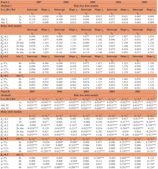
Table 3: The differences of the observed and theoretical parameters by direct estimation

Panel A 2007 2006 2005 2004 2003

Method 1 Risk free debt models

Lev1(Bv) Rel Intercept

γ0

Slope γ1 Intercept

γ0

Slope γ1 Intercept

γ0

Slope γ1 Intercept

γ0

Slope γ1 Intercept

γ0

Slope γ1

1a 0.118 0.008 0.109 0.012 0.094 0.013 0.072 0.011 0.065 0.008

Abs T_C 2a 0.118 0.012 0.109 0.019 0.094 0.022 0.071 0.020 0.065 0.013

Abs T_C 3a 0.117 0.008 0.109 0.013 0.094 0.015 0.071 0.014 0.065 0.009

Risky debt models

Intercept

γ₀ Slope γ1 Intercept γ₀ Slope γ1 Intercept γ₀ Slope γ1 Intercept γ₀ Slope γ1 Intercept γ₀ Slope γ1

β_D=0.2 1b 0.096 0.942 0.098 1.005 0.077 0.978 0.047 1.027 0.035 1.039

βD=0.3 1b 0.094 1.077 0.096 1.123 0.076 1.102 0.046 1.217 0.035 1.207

β_D=0.2 2b Abs 0.098 1.163 0.102 1.141 0.080 1.131 0.051 1.190 0.039 1.238 β_D=0.3 2b Abs 0.079 1.129 0.082 1.211 0.065 1.074 0.035 1.284 0.029 1.123 β_D=0.2 3b Abs 0.136 1.027 0.137 0.997 0.110 1.102 0.079 0.924 0.069 0.744

β_D=0.3 3b Abs 0.140 1.029 0.141 0.985 0.114 1.146 0.083 0.892 0.073 0.587

βD=0.2 Abs TC Intercept

γ0

Slope γ1 Intercept

γ0

Slope γ1 Intercept

γ0

Slope γ1 Intercept

γ0

Slope γ1 Intercept

γ0

Slope γ1

q=3% 4b 0.094 0.946 0.090 0.912 0.075 1.071 0.053 1.323 0.051 1.199

q=7% 4b 0.094 0.874 0.090 0.838 0.075 1.001 0.052 1.270 0.050 1.181

q=11% 4b 0.094 0.809 0.090 0.771 0.074 0.937 0.051 1.215 0.049 1.158

q=15% 4b 0.094 0.750 0.090 0.712 0.074 0.877 0.051 1.159 0.047 1.131

βD=0.3 Abs TC

q=3% 4b 0.093 1.057 0.089 1.028 0.075 1.190 0.054 1.466 0.056 1.132

q=7% 4b 0.093 0.976 0.089 0.941 0.074 1.111 0.053 1.413 0.054 1.137

q=11% 4b 0.093 0.901 0.089 0.863 0.074 1.037 0.052 1.354 0.053 1.134

q=15% 4b 0.093 0.833 0.089 0.792 0.074 0.967 0.051 1.292 0.051 1.124

Panel B 2007 2006 2005 2004 2003

Method1 Risk free debt models

Lev₁(Bv) Rel γ₀−γ₀* γ₁−γ₁* γ₀−γ₀* γ₁−γ₁* γ₀−γ₀* γ₁−γ₁* γ₀−γ₀* γ₁−γ₁* γ₀−γ₀* γ₁−γ₁* 1a 0.029*** −0.036*** 0.020*** −0.028*** 0.021*** −0.024*** 0.020*** −0.022*** 0.023*** −0.022***

Abs TC 2a 0.021*** −0.040*** 0.015*** −0.026*** 0.013*** −0.023*** 0.012*** −0.020*** 0.016*** −0.024***

Abs TC 3a 0.041*** −0.052*** 0.029*** −0.050*** 0.026*** −0.040*** 0.022*** −0.028*** 0.024*** −0.028***

Risky debt models

γ0−γ0* γ1−γ1* γ0−γ0* γ1−γ1* γ0−γ0* γ1−γ1* γ0−γ0* γ1−γ1* γ0−γ0* γ1−γ1*

β_D=0.2 1b 0.002 −0.058 0.006 0.005 −0.002 −0.022 −0.010*** 0.027 −0.013*** 0.039

β_D=0.3 1b −0.003 0.077 0.001 0.123 −0.006 0.102 −0.015*** 0.217** −0.016*** 0.207**

β_D=0.2 2b Abs −0.003 0.163** 0.003 0.141* −0.005 0.131 −0.013*** 0.190*** −0.015*** 0.238***

β_D=0.3 2b Abs −0.024*** 0.129 −0.019*** 0.211* −0.022*** 0.074 −0.031*** 0.284** −0.028*** 0.123

β_D=0.2 3b Abs 0.050*** 0.027 0.053*** −0.003 0.038*** 0.102 0.025*** −0.076 0.024 −0.256***

β_D=0.3 3b Abs 0.052*** 0.029 0.056*** −0.015 0.040*** 0.146 0.028*** −0.108 0.026*** −0.413***

β_D=0.2 Abs T_C γ₀−γ₀* γ₁−γ₁* γ₀−γ₀* γ₁−γ₁* γ₀−γ₀* γ₁−γ₁* γ₀−γ₀* γ₁−γ₁* γ₀−γ₀* γ₁−γ₁*

q=3% 4b 0.009*** −0.054 0.008* −0.088* 0.004 0.071 0.000 0.323*** 0.006 0.199***

q=7% 4b 0.010*** −0.126* 0.009* −0.162*** 0.006 0.001 0.000 0.270*** 0.006 0.181***

q=11% 4b 0.012*** −0.191*** 0.011*** −0.229*** 0.006 −0.063 0.000 0.215*** 0.006 0.158**

q=15% 4b 0.013*** −0.250*** 0.012*** −0.288*** 0.007 −0.123*** 0.001 0.159*** 0.005 0.131*

β_D=0.3 Abs T_C

q=3% 4b 0.006 0.057 0.005 0.028 0.002 0.190*** −0.001 0.466*** 0.009 0.132

q=7% 4b 0.008 −0.024 0.006 −0.059 0.003 0.111 0.000 0.413*** 0.008 0.137*

q=11% 4b 0.009 −0.099 0.008* −0.137*** 0.004 0.037 0.000 0.354*** 0.008 0.134*

q=15% 4b 0.011*** −0.167*** 0.009*** −0.208*** 0.005 −0.033 0.000 0.292*** 0.007 0.124*

while the bottom part presents the findings of the statistical t test employed for the differences between the theoretical and observed regression parameters. Note that all of the regression tables report the results for a market premium estimate of 6%, but the results remain essentially unchanged when we use two 5% and 7%.

In accordance with the theoretical predictions, the relationship between K_E and L is positive in all of the regression equations estimated. Table 2 demonstrates a positive relationship between

financial leverage (L) and the K_E for the results of all of the regressions. As the last line of each model in Table 2 indicates, the significance level of γ₁ (the slope) is ≤1% for each of the sample years of the sample and for each of the L estimates. Although not reported in the tables, γ₁ (the intercept) in the various equations is also statistically significant. Thus, the relationship between K_E and L is positive and statistically significant for the values of all of the variables in the regression equations: The corporate tax rate, personal tax rate, debt beta, and the bankruptcy costs.

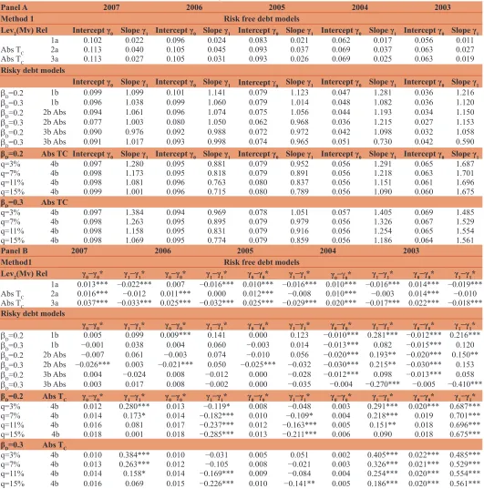
Table 4: The differences of the observed and theoretical parameters by direct estimation

Panel A 2007 2006 2005 2004 2003

Method 1 Risk free debt models

Lev2(Mv) Rel Intercept γ0 Slope γ1 Intercept γ0 Slope γ1 Intercept γ0 Slope γ1 Intercept γ0 Slope γ1 Intercept γ0 Slope γ1

1a 0.102 0.022 0.096 0.024 0.083 0.021 0.062 0.017 0.056 0.011

Abs T_C 2a 0.113 0.040 0.105 0.045 0.093 0.037 0.069 0.037 0.063 0.027

Abs T_C 3a 0.113 0.027 0.105 0.031 0.093 0.026 0.069 0.025 0.063 0.019

Risky debt models

Intercept γ0 Slope γ1 Intercept γ0 Slope γ1 Intercept γ0 Slope γ1 Intercept γ0 Slope γ1 Intercept γ0 Slope γ1

β_D=0.2 1b 0.099 1.099 0.101 1.141 0.079 1.123 0.047 1.281 0.036 1.216

β_D=0.3 1b 0.096 1.038 0.099 1.060 0.079 1.014 0.048 1.082 0.036 1.120

β_D=0.2 2b Abs 0.094 1.061 0.096 1.074 0.075 1.056 0.044 1.193 0.034 1.150

βD=0.3 2b Abs 0.077 1.003 0.080 1.050 0.062 0.968 0.036 1.215 0.027 1.153

β_D=0.2 3b Abs 0.090 0.976 0.092 0.988 0.072 0.972 0.042 1.098 0.032 1.058

β_D=0.3 3b Abs 0.091 1.017 0.093 0.998 0.074 0.965 0.051 0.730 0.042 0.590

β_D=0.2 Abs TC Intercept γ₀ Slope γ₁ Intercept γ₀ Slope γ₁ Intercept γ₀ Slope γ₁ Intercept γ₀ Slope γ₁ Intercept γ₀ Slope γ₁

q=3% 4b 0.097 1.280 0.095 0.881 0.079 0.952 0.056 1.291 0.065 1.687

q=7% 4b 0.098 1.173 0.095 0.818 0.079 0.891 0.056 1.218 0.063 1.701

q=11% 4b 0.098 1.081 0.096 0.763 0.080 0.837 0.056 1.151 0.061 1.696

q=15% 4b 0.099 1.001 0.096 0.715 0.080 0.789 0.056 1.090 0.060 1.675

β_D=0.3 Abs TC

q=3% 4b 0.097 1.384 0.094 0.969 0.078 1.051 0.057 1.405 0.069 1.485

q=7% 4b 0.098 1.263 0.095 0.895 0.079 0.979 0.056 1.326 0.067 1.529

q=11% 4b 0.098 1.158 0.095 0.831 0.079 0.916 0.056 1.254 0.065 1.554

q=15% 4b 0.098 1.069 0.095 0.774 0.079 0.859 0.056 1.186 0.064 1.561

Panel B 2007 2006 2005 2004 2003

Method1 Risk free debt models

Lev2(Mv) Rel γ0−γ0* γ1−γ1* γ0−γ0* γ1−γ1* γ0−γ0* γ1−γ1* γ0−γ0* γ1−γ1* γ0−γ0* γ1−γ1*

1a 0.013*** −0.022*** 0.007 −0.016*** 0.010*** −0.016*** 0.010*** −0.016*** 0.014*** −0.019***

Abs T_C 2a 0.016*** −0.012 0.011*** 0.000 0.012*** −0.008 0.010*** −0.003 0.014*** −0.010

Abs T_C 3a 0.037*** −0.033*** 0.025*** −0.032*** 0.025*** −0.029*** 0.020*** −0.017*** 0.022*** −0.018***

Risky debt models

γ₀−γ₀* γ₁−γ₁* γ₀−γ₀* γ₁−γ₁* γ₀−γ₀* γ₁−γ₁* γ₀−γ₀* γ₁−γ₁* γ₀−γ₀* γ₁−γ₁*

β_D=0.2 1b 0.005 0.099 0.009*** 0.141 0.000 0.123 −0.010*** 0.281*** −0.012*** 0.216***

β_D=0.3 1b −0.001 0.038 0.004 0.060 −0.003 0.014 −0.013*** 0.082 −0.015*** 0.120

β_D=0.2 2b Abs −0.007 0.061 −0.003 0.074 −0.010 0.056 −0.020*** 0.193** −0.020*** 0.150**

β_D=0.3 2b Abs −0.026*** 0.003 −0.021*** 0.050 −0.025*** −0.032 −0.030*** 0.215** −0.030*** 0.153

β_D=0.2 3b Abs 0.004 −0.024 0.008 −0.012 0.000 −0.028 −0.012*** 0.098 −0.013*** 0.058

β_D=0.3 3b Abs 0.003 0.017 0.008 −0.002 0.000 −0.035 −0.004 −0.270*** −0.005 −0.410***

βD=0.2 Abs TC γ0−γ0* γ1−γ1* γ0−γ0* γ1−γ1* γ0−γ0* γ1−γ1* γ0−γ0* γ1−γ1* γ0−γ0* γ1−γ1*

q=3% 4b 0.012 0.280*** 0.013 −0.119* 0.008 −0.048 0.003 0.291*** 0.020*** 0.687***

q=7% 4b 0.014 0.173* 0.014 −0.182*** 0.010 −0.109* 0.004 0.218*** 0.019 0.701***

q=11% 4b 0.016 0.081 0.017 −0.237*** 0.012 −0.163*** 0.005 0.151** 0.018 0.696***

q=15% 4b 0.018 0.001 0.018 −0.285*** 0.013 −0.211*** 0.006 0.090 0.018 0.675***

βD=0.3 Abs TC

q=3% 4b 0.010 0.384*** 0.010 −0.031 0.005 0.051 0.002 0.405*** 0.022*** 0.485***

q=7% 4b 0.013 0.263*** 0.012 −0.105 0.008 −0.021 0.003 0.326*** 0.021*** 0.529***

q=11% 4b 0.014 0.158* 0.014 −0.169*** 0.009 −0.084 0.004 0.254*** 0.020*** 0.554***

q=15% 4b 0.016 0.069 0.015 −0.226*** 0.010 −0.141** 0.005 0.186*** 0.020*** 0.561***

Table 4 presents the observed parameters obtained by a direct regression of each model and their differences from their counterparts’ theoretical values. The financial leverage measure used here is Lev2(Mv) Rel. Panel A presents the observed parameters and Panel B presents the differences test conducted for each value. Each row specifies the relevant model and the

Furthermore, the findings are similar when the corporate tax variable is measured using either the absolute or relative method, or when the β_D estimate is 0.3, 0.2 or 0.1.

One of our important results is that the relationship between L and K_E, as represented by R-squared, is much higher for the risky debt models (Case B) than for the risk free models (Case A). For the perfect capital market case, the mean R-squared value increases from 19.5% for Model (1a) to 41.7% for Model (1b). Similarly, in Model (3a), that includes corporate and personal taxes case, the mean R-squared value increases from 18.9% for the risk free case to 54.7% in the risky debt case. Comparing Model (2b) and Model (2a) yields similar results. The R-squared value increases from 18.5% for the risk free case to 54.7% in the risky debt case. Interestingly, the highest R-squared values are evident in Model (4b), which incorporates both taxes and bankruptcy costs. The mean R-squared value is 66.3%.

Another important finding is that the R-squared value is higher for all of the models based on market measures rather than book measures of the financial leverage. For example, (though not reported here), the market based relative Lev₄ measure, not reported here, yields an R-squared value of 19.8% compared with 11.3% for the book based relative Lev₃ measure. This result generally holds for corresponding book and market L measures.

To summarize, all of the empirical results in each model tested point to a positive relationship between the K_E and financial leverage regardless of the measures used for the key variables. Second, the coefficient of determination (R2_{) increases dramatically in}

the transition from risk free debt models to their parallel risky debt ones. Third, the market measures of financial leverage tend to generate a higher coefficient of determination for the goodness of fit. All of the tests we conducted confirm this result.

5.3. Comparative Analysis

As discussed above, our study yields three main findings: (1) The relationship between K_E and Lis positive regardless of the specific measures of the various variables, (2) The R-squared value is substantially higher in the risky debt models than in the risk free debt models and (3) The market measures of L tend to generate higher R-squared values than the book measures of L.

Our next task is to compare the observed γ₀ and γ₁ values as given by the OLS results with their theoretical counterparts given by the direct values of the variables such as tax rates, and bankruptcy costs. The failure to reject the null hypothesis means an insignificant gap between the theoretical and observed parameters, which is in fact, the result needed to validate a model. The interpretation of the null hypothesis is that the theoretical model holds true because the observed parameter is statistically not different from it. Such a comparison will allow us to determine whether the risk free or risky debt models accord most closely with the actual K_E–L relationship. We follow the standard procedures related to the slope γ₁ and the intercept γ₀ for testing the hypotheses. First, we specify the null and alternative hypotheses. According to the null hypothesis, γ₁ equals a theoretical value that we will call γ₁*. The alternative hypothesis is that γ₁ is different from the

theoretical value γ₁*. Second, we calculate the statistic T using Equation (18):

1 1 1 1

1 2

stat

* *

T

Se( ) MSE

( Xi X )

γ γ γ γ

γ

− −

= =

−

(18)

where, γ₁ is the observed slope obtained in the regression analysis, γ₁* is the theoretical value of the slope according to each model, and MSE is the error mean sum of squares, which is calculated by dividing the sum of squares within the groups by the error degrees of freedom. The denominator of MSE is the total sum of squares scaled by its degrees of freedom, and finally, Se (γ₁) is the standard error of the observed slope γ₁.

Similarly, the t-test for the intercept (γ₀) involves two hypotheses. According to the null hypothesis, γ₀ equals the theoretical intercept γ₀*. The alternative hypothesis is that γ₀ is different from the theoretical value γ₀*. Second, we calculate the statistic T using Equation (19):

0 0 0 0

2

0 2

* *

( ) 1

( )

stat T

Se X

MSE

n Xi X

γ γ γ γ

γ

− −

= =

× +

Σ −

(19)

where γ₀ is the observed slope obtained in the regression analysis, γ₀* is the theoretical value of the intercept according to each model, MSE is the error mean sum of squares, which is calculated by dividing the sum of squares within the groups by the error degrees of freedom, and finally, S_e (γ₀) is the standard error of the observed intercept γ₀. As stated earlier, Tables 3 and 4 present the findings of the statistical t-test that was established for the differences between the theoretical and observed regression slope and intercept for the direct estimation of each model. Due to the vast number of iteration and the similarity of results, we report only the results obtained using the Relative Lev₁ and Lev₂.

The theoretical intercept (γ₀*) and slope(γ₁*) for each of the risk free and risky debt models in the context of the K_E−L relationship are derived according to the hypotheses formulated in Section 3. Due to the vast number of possible iterations, we present just the estimated theoretical and observed regression coefficients according to the absolute corporate tax measure when the mean value of β_D is 0.2 and 0.3, and the bankruptcy costs are 3%, 7%, 11% and 15%. We also report the results for the Lev₁(Bv) Rel

and Lev₂(Mv) Rel financial leverage measures. Using Lev₃(Bv)

Abs and Lev₄(Mv) Abs yield results that remain the same but are not reported here. An illustration for the construction of the theoretical coefficients is given below. For example, Model (2a) is formulated as:

K_E=K_U+[(K_U–r)(1−T_C)L] (2a)

And the estimated regression is: