Is the Soil Frozen, or Not? An Algorithm Using Weather Records

VOL. 14, NO. 6

limpaloased by the U. S. Pupa rtroont of Agriculture Fat Official Use

WATER RESOURCES RESEARCH DECEMBER 1978

K//

Is the Soil Frozen or Not?

An Algorithm Using Weather Records

J. W. CARY

USDA Snake River Conservation Research Center, Kimberly, Idaho 83341

G. S. CAMPBELL

Washington State University, Pullman, Washington 99164

R. I. PAPENDICK

USDA Science and Education Administration, Pullman, Washington 99164

Frozen soil water is important in hydrologic events because it reduces water infiltration. The presence of soil ice can be predicted reasonably well from detailed knowledge of the soil and microclimatic variables, but this type of information is generally unavailable. Consequently, the purpose of this study was to start with fundamental relations and see how well frozen soil conditions could be identified from daily weather station records of maximum-minimum temperatures, solar radiation, and snowfall. Two relations were developed, one based on the soil-atmosphere energy budget and the other on the heat flux across the soil surface layer. Conceptually, the two equations may be used together to give daily snowrnelt as well as soil thawing and freezing rates, but in practice, the snowmen prediction is probably not yet accurate enough for most practical applications. The simpler equation, describing the heat flux in the soil surface, does not require solar radiation input, yet it gave fair predictions of frozen soil on five diverse sites studied in the Palouse region of eastern Washington. Both approaches require only a single constant that accounts for individual site conditions such as slope, aspect, cover, and soil properties.

passed from the fluid in the tube past a stopper in the cap to the atmosphere. This initiated ice nucleation and reduced su-percooling of the fluid. Thin-walled rubber tubing was im-bedded in sand in the center of the tube and vented at the bottom to absorb the volume increases from freezing.) Maxi-mum and miniMaxi-mum air temperatures and precipitation were measured at a weather station 1 km from the sites. Solar radiation was measured on the Washington State University campus 10 km distant. All data were obtained with standard commercial instruments, except the soil heat flux meters, which are described by Fuchs and Hadas [1973].

The winter climate of eastern Washington is humid with mixed rain-snow precipitation and interspersed periods of freezing-thawing weather. Frost depth is usually less than 30 cm, but soil may freeze and then completely thaw several times during the winter, thaw often being accompanied by rain or melting snow.

INTRODUCTION

Soil ice reduces the infiltration of water. Consequently, it is an important factor in predicting floods, seasonal water sup-plies, and soil erosion from runoff. If detailed information on soil properties and microclimate is available, reasonably good estimates of soil freezing and thawing can be made [Dempsey and Thompson, 1969]. More often, however, one has only a general description of the site and records of daily precipi-tation and maximum-minimum temperatures from a regional weather station. Occasionally, daily values of solar radiation are also available. Consequently, the objective of this study was to develop, from fundamental considerations, methods for predicting when the soil was frozen using daily weather station records of temperature, solar radiation, and precipitation.

METHODS

Five sites, each representing a different slope or aspect of the diverse Palouse topography in the Pacific Northwest, were selected for study. Characteristics of these sites, located on the Palouse Conservation Field Station near Pullman in eastern Washington, are listed in Table 1. The soil was Palouse silt loam or a closely related series (Pachic Ultic Haploxerolls), formed from loess with deep, permeable profiles. At the onset of freezing weather in December the soil water content was near field capacity in the surface 20-30 cm and dry to the plant-wilting point below this level to a depth of 1.5 m.

Thermocouples and heat flux meters were installed on all the sites, and measurements were made either automatically at 2-hour intervals or manually during periods of interest. Frost tubes similar to those described by Rickard and Brown [1972] were installed on all sites. (The frost tubes were modified near the end of the experiment with a small cotton thread that

This paper is not subject to U.S. copyright. Published in 1978 by the American Geophysical Union.

Paper number 8W0614. 11 I 7

THEORY

M= (G. + LIM (1)

Concepts

1118 CARY ET AL.: FROZEN SOIL

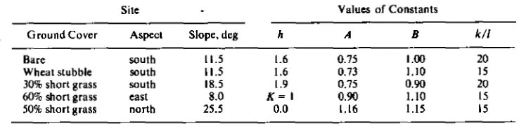
TABLE 1. Description of Study Sites and Values of Constants Used to Calculate Frost Conditions

Site Values of Constants

Ground Cover Aspect Slope, deg h A B kIl

Bare south 11.5 1.6 0.75 1.00 20

Wheat stubble south 11.5 1.6 0.73 1.10 15

30% short grass south 18.5 1.9 0.75 0.90 20

60% short grass east 8.0 K = I 0.90 1.10 15

50% short grass north 25.5 0.0 136 1.15 15

where

ill <

0 indicates soil frozen and

M

0 indicates soil not frozen. In this relation,

it

indicates the day beginning with the soil near 0°C.

G.

is the daily average soil heat flux downward across the surface, and upn the daily soil heat flux upward from subsoil layers into the zone susceptible to freezing. The problem thus becomes one of evaluating (1) from weather station records of daily temperature extremes, solar radiation, and snowfall.

Values of up„ determined from measurements of thermal conductivity and soil temperature gradients were relatively small, of the order of 2 W m- 5 . For this study the empirical relation

up„ — 2.5 sin

(J +

80) (2)

where J is the Julian date, gave values of mean daily upward soil heat flux that followed the experimental measurements reasonably well.

The downward soil heat flux

G

may be estimated in two ways: (1) from the net energy exchange between the soil sur-face and the atmosphere and (2) from the heat conducted across the soil surface.

The daily heat conducted across the soil surface is approxi-mately

G. = (k/1)(T„ —

T0 ) (3)

where

T,

is the average soil surface temperature,

T„

is the average soil temperature at some shallow depth and

k

is the average soil thermal conductivity over

1.

Soil heat flux from the energy balance approach is given by

G = R. — XE H (4)

where

R.

is the net radiation, XE is the heat associated with the evaporation of water, and

H

is the sensible heat exchanged between the surface and the air. During the cold season, net radiation often dominates this relation (Granger

et a!.,

1977]; however, when the weather is overcast or foggy, the sensible heat exchange may be important. The evaporation term XE generally gives a net soil heat loss, but important exceptions do occur when the relative humidity is high; i.e., the presence of warm, moist air may result in the gain of heat by frozen soil or snow. Because the surface temperature of snow or ice does not rise above freezing, air dew-point temperatures above 0°C lead to condensation on snow or frozen surfaces with large releases of latent heat. A warm rain falling on snow causes rapid melt, not because of the energy carried by the raindrops themselves but because the rain favors a dew-point temperature above freezing. Water vapor condensing on the snow releases enough heat to melt 7 times the vapor's own weight of

ice.

Heat gained by vapor condensation is of the same order of magnitude as sensible heat gained from the air when the dew-point temper-ature is near the air tempertemper-ature and above freezing (see, for example, the last two terms in (5)).

Soil Heat Flux From the Energy Balance

The average daily soil heat flux may be estimated from (4) by using daily air temperature extremes, solar radiation, snow-fall, and several assumptions that deserve critical consid-eration.

Equation (4) may be written in more detail

[Campbell,

1977, p. 61] as

G

LA

E p.C„ AT

r r (5)

where the terms correspond to those in (4) and definitions and dimensions of the variables are as follows:

a

soil heat flux (downward flow positive), W m- 5;

R„

net radiation, W m- 1;

A latent heat of vaporization, J g-';

Ap

difference in water vapor concentration between the air at the soil surface and the air 2 m above the surface, g m- 5;

p„

density of air, g m- 5;

Cp specific heat of air, J g- °C- 1 ;

A

T

difference between the soil surface temperature and the temperature of the air 2 m above the surface, °C; r transfer coefficient, s m-'.

Equation (5) is an instantaneous relationship; i.e., the true average values of XE and

H

for a time period of a few hours can only be approximately calculated from time average values of AT, Ap, and

r

because these variables change with time but not necessarily in phase with each other. Nevertheless, it was assumed that (5) holds, using daily mean values of all vari-ables.

Net radiation may be expressed as

R. =

(1 — a)S,'

+ o(T 14t, —

7,1t1) (6)

where

a

is the shortwave reflectivity,

a

is the Stephan-Boltz-mann constant, St ' is total shortwave radiation,

T,'

and

T,'

are the air and soil surface temperatures in degrees Kelvin, and

E is emissivity, E ar being the total incoming long-wave radiation and a. the outgoing long-wave radiation from the soil.

Using the approximation

T,i4 = (Tar +

A Tr

T,14 +

47'n ' 5 A

T

(7)

and Penman's transform

[Campbell,

1977, p. 120], (5) becomes

Gn

= R.' — AT (4oe„T," +

_r

+

_r

— (Pal

_r

— Pa)

—

CARY ET AL.: FROZEN SOIL 1119

where all quantities are now taken as daily averages, In (8),

R.' defined for convenience in programing as equal to R. + 4E. T." AT;

slope of the saturated vapor density curve;

Pe: saturated water vapor concentration at temperature T.;

daily average heat flux that will be required to supply latent heat eventually to melt daily snowfall.

When snow is present, G. in (8) is the heat flux across the snow-atmosphere interface.

The heat and vapor transfer coefficient for a nearly smooth surface is r = 700/fi, where a is the average wind speed in meters per second [Campbell, 1977, p. 138]. In this study, r =

300 s m-' was chosen on the basis of average wind speeds, and e. = 0.98 on the basis of a typically moist soil surface.

Using the daily minimum temperature T,,, as an estimate of the dew-point temperature,

Pa' - Pa = 0.012(7'2 - T„,2) + 0.34(T. - T„,) (9)

where T. is the mean daily air temperature in degrees Celsius, Equations (9) and (14) are best-fit quadratic relations describ-ing data given by Campbell [1977, p. 150]. Similarly, in (8), s

can be represented as

s = 5.6 X 10-72 + 0.02 7; + 0.34 (10)

when temperatures are within a few degrees of zero.

Taking a = 0.1, (6) may be rearranged for any land slope and aspect as

= 0.9[S. + K(S, - S.)] + - 0.98) (11)

where S. is the diffuse shortwave radiation and S t the total shortwave radiation over a level surface. Daily values of Se

may be calculated from the average of hourly values given by

Campbell's [1977] equation (5.11). A constant daily value of 25 W m-2was used for Sd, which agreed with measured values of

S, on winter days with heavy overcast. The factor K corrects for the effects of slope and aspect on the interception of direct shortwave radiation. Daily values of K at various latitudes can be interpolated from tables published by Buffo et al. [1972] and fitted to equations of the type

K = h[sin (J + b0)]112 (12)

where.] is the Julian date and bais the phase factor, taken as 95 for south slopes at this location. Values of h for each of the study sites are given in Table 1.

Campbell gives an equation [Campbell, 1977, p. 58, equation (5.14)] for estimating c.e, which was modified as

= 0.58p.°1" + (A - -vk ) (0.97 - 0,58p.°•1") (13) where

p. = 0.0127;2 + 0.34T„, + 4.82 (14)

in the neighborhood of 0°C, when T. is a valid estimate of the dew-point temperature. Values for the potential shortwave radiation s,„ are given by List [1951] and expressed by the relation

St. = ai sin (I + b1) + c: (15)

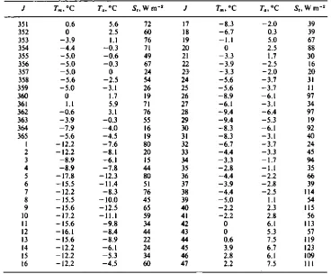
TABLE 2, Weather Station Measurements During the Study Period

°C T„, °C S„W rn- 2

J

7-„„ °C r„, °C S,, W m-2

351 0.6 5.6 72 17 -8.3 -2.0 39

352 0 2.5 60 18 -6.7 0.3 39

353 -3.9 1.1 76 19 -1.1 5.0 67

354 -4.4 -0.3 71 20 0 2.5 88

355 -5.0 -0.6 49 21 -3.3 1.7 30

356 -5.0 -0.3 67 22 -3.9 -2.5 16

357 -5.0 24 23• -3.3 -2.0 20

358 -5.6 -2.5 5.4 24 -5.6 -3.7 31

359 -5.0 -3.1 26 25 -5.6 -3.7 11

360 0 1.7 19 26 -8.9 -6.1 97

361 1.1 5.9 71 27 -6.1 -3.1 34

362 -0.6 3.1 76 28 -9.4 -6.4 97

363 -3.9 -0.3 55 29 -9.4 -5.3 19

364 -7.9 -4.0 16 30 -8.3 -6.1 92

365 -5.6 -4.5 19 31 -8.3 -3.1 40

-12.2 -7.6 80 32 -6.7 -3.7 24

2 -12.2 -8.1 20 33 -4.4 -3.3 45

3 -8.9 -6.1 15 34 -3.3 -1.7 94

4 -8.9 -7.8 44 35 -2.8 -1.1 35

5 -17.8 -12.3 80 36 -4.4 -2.2 66

6 -15.5 -11,4 51 37 -3.9 -2,8 39

7 -12.2 -8.3 76 38 -4.4 -2.5 114

8 -15.5 -10.0 45 39 -5.0 1.1 54

9 -15.6 -12.5 65 40 -2.2 2.3 115

10 -17.2 -11.1 59 41 -2.2 2.8 56

11 -15.6 -9.8 34 42 0 6.1 113

12 -16.1 -8.4 44 43 0 5.3 57

13 -15.6 -8.9 22 44 0.6 7.5 119

14 -12.2 -6.1 24 45 3.9 6.7 123

15 -12.2 -5.3 34 46 2.8 6.1 109

16 -12.2 -4.5 60 47 2.2 7.5 111

356

JULIAN DAY

10 20

100

20

1-1

14 • •••,d4

•

40

60

—100 N

E

3

—200

—300

5 20 — 100

40

JULIAN DAY 10 20

356

100

60 — 300

E 3

1120 CARY ET AL,: FROZEN SOIL

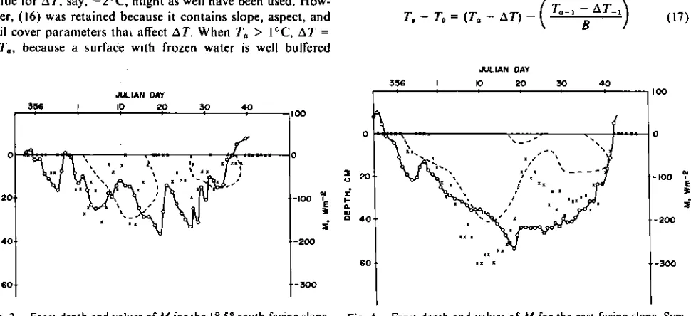
Fig. I. Frost depth and sum of the soil heat flux deficits M for the

bare south-facing slope. The dashed line shows the depth of frost Fig. 3. Frost depth and values of M for the north-facing slope. penetration, the solid line shows M From (8), and the crosses give M Symbols are the same as those in Figure 1.

from (18).

where a, = 150, b, = 280, and c 1 230 for our study location. The term A – (S,ISio) corrects long-wave radiation for condi-tions different from a clear sky forming a complete hemisphere over the site. The constant A is a site factor with values near 1 that are sensitive to rough terrain and vegetative cover. Since A is chosen for each site to give the best fit between observed and predicted dates of soil freezing and thawing, it includes the effects of soil physical properties as well as a correction for all bias in the analysis resulting from assumptions and non-random measurement errors. Values of A for the five study sites are listed in Table 1.

One major difficulty with this energy balance approach is specifying accurate daily averages of AT. In this study, values of q T and R5 integrated over 2-hour time periods were

mea-sured on the bare south-facing site using a long-wave and a net radiometer. A linear correlation of these data led to the empir-ical relation

AT = –0.03R„' – 1 (16)

with a correlation coefficient r2 = 0.33 between observed and measured values of T. The r2 value suggests that a constant value for AT, say, –2°C, might as well have been used. How-ever, (16) was retained because it contains slope, aspect, and soil cover parameters that affect A T. When To > 1°C, q T = –To , because a surfaCe with frozen water is well buffered

against temperatures above 0°C. This relation was included in the program with (16); i.e., the calculations were made on a hand-held programmable calculator,

Equations (9)–(16) and the associated assumptions allow one to estimate the average daily soil heat flux from (8) using the weather station data given in Table 2. The result can be used with (2) in (1) to predict whether or not the soil is frozen, provided there is no snow cover. Positive values of Al indicate that the soil is thawed and the snow is melted. When M is negative, the amount of frozen water in the snow cover must be known before conclusions concerning the presence of soil ice can be reached.

Soil Heat Flux From the Surface Layer Approach

Equation (3) suggests a simple way to estimate daily soil heat flux from weather station measurements of daily mean temperature and snowfall. The average soil temperature To a

few centimeters beneath the surface will be proportional to the previous day's surface temperature. Combining this with the definition of AT gives T, = (T5_, – A T _,)/1- 1 , so that the temperature difference term in (3) becomes

— A T_,)

B

To = (To — AT) ( (17)

•

%RAJAH DAY

10 20

a E

CARY ET AL.: PROZEN SOIL 1121

Fig. 5. Frost depth and values of M for the straw stubb e plot. Symbols are the same as those in Figure 1.

where the - I subscript indicates the previous day and B is the proportionality constant. Assuming that AT - AT_ 1 = 0 and

B is near 1, (3) becomes approximately

k 12

08)

G„ = T T.

-+ N I

where a damping term for snow cover l - [1,1(12 + has been included with the snow depth 1P , Since there was no significant snow cover during this study, the reader is referred to the work of Anderson [1976] for information on choosing a proper value for the constant N. The depth I was in the range 5-10 cm for these study sites. When T„,_, > 0, is taken as zero in (18) because of the presence of ice in the soil. Likewise, when snow is present, the program must set the upper limit at T, at zero. When (18) is used to evaluate (1), the freeze and thaw dates are determined by the value of B, while deter-mines only the amplitude of M. When Al > 0, M was taken as zero in our program because the damping depth of unfrozen soil is much greater than it is when ice is present. Thus/should

increase, while k generally decreases because of drainage away from the surface. The result is a decrease in G. after the soil thaws.

RESULTS

The weather station data (Table 2) were used with the individual site constants (Table 1) to calculate values of Al

from (l) as a function of time. The results for each site are presented in Figures 1-5.

Values of M, using (8), did not predict the soil thaw periods between days 14 and 25 (Figures 1 and 2), nor did the curves produced by this algorithm match the depth of freezing curves very well after day 15 for any of the sites. Of course, the depth of freezing is not a unique function of the soil heat flux deficit because only part of the soil water freezes at 0°C. For ex-ample, in this soil, when the temperature falls from -0.1° to -1°C, an additional 12% of the soil water freezes, and the heat released will correspond to a daily average flux of 40 W m- 2 for each centimeter of water frozen. With an additional drop from -1° to -8°C, another 5% of the soil water freezes [Cary and Mayland. 1972]. Obviously, the heat flux deficit M may vary by 50 W m-2 or more just because of soil temperature fluctuations near the surface without any change in frost pene-tration. The soil water content is also an important factor in the relation between freezing depth and values of M. The

scales in Figure 1 were chosen so the freezing depth would approximately correspond to values of M. Owing to greater soil water contents, values of M in Figures 3-5 should be lower than the freezing curves but still approximate their shapes. The daily average heat flux measurements from transducers on the bare plot followed the freezing depth curve closely for the first 35 days but then did not predict the brief period of thawing that followed, possibly because of a faulty electrical circuit. A linear regression between the measured and the predicted heat flux from (8) had a correlation coefficient of r2 = 0.53 during the first 35 days.

Values of Al based on (18) predicted frozen soil better than those from (8), even though (18) does not include measure-ments of solar radii tion. The correlation coefficient DIG. from (18) with measured soil heat flux on the bare site was r2 = 0.61. As was pointed out by Zuze! and Cox [1975], air temperature is the best single parameter that one has for integrating the characteristics of microclimate. The most obvious error caused by the omission of St in the development of (18) is seen in Figure 3, where freezing of the north slope.was not predicted until 10 days after it actually occurred. The values of M using

G„ from (18) did not become negative at first because average daily air temperatures were above freezing; but the soil, which was in the shade of the north slope, was freezing from long-wave radiation loss to clear skies. The effects of radiation could be included in (18) by starting with (17) and writing AT = f(St ) and AT_ 1 = f(S,_,). This was not attempted here because AT was measured only on the bare, south-facing site. A better method for finding AT = g(S„ T5 , T„,) (site proper-ties) is needed for both (8) and (17). Outcalt et al. [19751 gave a numerical procedure for calculating average daily AT values at the snow-air interface. While their prediction of snowmelt was good, they did not report measurements of AT for comparison with calculated values. Smith and Tvede [1977] used the ap-proach of Outcalt et al. to predict freeze-thaw dates and frost penetration under bare highways with no evaporation of wa-ter. They felt that this finite difference approach reproduced daily surface temperatures within 1° or 2° from daily air temperature, solar radiation, cloud cover, wind speed, air pres-sure, and some knowledge of the soil properties. Their predic-tions of freezing and thawing under several highways appear to have about the same accuracy as those in the study reported here, Anderson [1976] also presents a procedure for calculating AT values of a snow surface. His calculated values agreed within 1° or 2°C with those measured, agreement which is of about the same order of magnitude as our measured daily averages of AT values on the bare soil site. Other methods for finding AT of bare soil surfaces are available but require more detailed weather data than we use here [Van Baud and Hillel,

1976].

APPLICATIONS

Since daily weather station records are available in many areas, ( I) may be useful for analyzing data from past hydro-logic events when the interpretation depends on knowledge of whether or not the soil was frozen. Equation (18) is obviously the preferred method for finding daily average values of G. to be used in (I) when only limited weather station records are available. However, calculation of G. from (8) is of more than passing interest because the difference in values of Al from (8)

1122 CARY ET AL.; FROZEN SOIL

(IS) could lead to a useful algorithm for predicting snowmelt as well as freezing and thawing of the soil.

Both (8) and (18) require a site constant which must be determined individually. Frozen soil data for this purpose can be obtained with frost tubes or thermocouples. If resources are available to make additional measurements other than T., T„„ and SI , soil heat flux at representative sites will be a good choice for many purposes. Heat flux meters placed just be-neath the soil surface and just below the zone of deepest frost penetration will give values for M from a voltage integrator.

The soil heat flux deficit M may be used to estimate the depth of frost penetration if one also knows the soil water release curve as well as the water content and soluble salt distribution with depth [Cary and Mayland, 1972]. In like man-ner, if one has this information on the soil properties and is measuring the frost penetration with frost tubes or thermo-couples, M can be estimated. These values of M might then be used in the algorithms presented here to predict the type of weather that must occur before the soil will thaw, a key factor in flood and water storage forecasting.

REFERENCES

Anderson, E. A., A point energy and mass balance model of a snow cover, NOAA Tech. Rep. N WS 19, U.S. Dep. of Commer,, Boulder, Colo., 1976.

'Buffo, J., L. J. Fritschen, and J. L. Murphy, Direct solar radiation on various slopes from 0 to 60 degrees north latitude, Forest Serv. Res.

Pap. PNW-142, 74 pp., U.S. Dep. of Agr., Portland, Oreg., 1972.

Campbell, G. S., An Introduction to Environmental Biophysics, 159 pp., Springer, New York, 1977.

Cary, J. W., and H. F. Mayland, Salt and water movement in unsatu-rated frozen soil, Soil Sci. Soc. Amer. Proc., 36, 549-555, 1972. Dempsey, B. J., and M. R. Thompson, A heat-transfer model for

evaluating frost action and temperature related effects in multi-layered pavement systems, U.S. Dep. Transp. Proj. IHR-401, l99

pp., Dep. of Civil Eng., Eng. Exp. Sta., Univ. of Ill., Urbana, 1969. Fuchs, M., and A. Hadas, Analysis of the performance of an improved sail heat flux transducer, Soil Sci. Soc. Amer. Proc., 37, 173-175,

1973.

Granger, R. J., D S. Chanarsyk, D. M. Male, and D. 1. Norm, Thermal regime of a prairie snow cover, Soil Set Soc. Amer. J., 41, 839-842, 1977.

List, R. J.. Smithsonian Meteorological Tables, vol. 114, 527 pp., Smithsonian institution Press, Washington, D. C., 1951.

Outcalt, S. 1., C. Goodwin, G. Weller, and J. Brown, Computer simulation of the snowmelt and soil thermal regime at Barrow, Alaska, Water Resour. Res., 11, 709-715, 1975.

Rickard, W., and J. Brown, The performance of a frost-tube for the determination of soil freezing and thawing depths, Soil Set. 113,

149-154, 1972.

Smith, M. W., and A. Tvede, The computer simulation of frost pene-tration beneath highways, Can. Geotech. J., 14; 167-179, 1977. Van Bavel, C. H. M., and D. 1. Hillel, Calculating potential and actual

evaporation from a bare soil surface by simulation of concurrent flow of water and heat, Agr. Meteorot, 17, 453-476, 1976. Zuzel, J. F., and L. M. Cox, Relative importance of meteorological

variables in snowmelt, Water Resour. Res., 11, 174-176, 1975. (Received March l5, 1978;