The Thirty-Third AAAI Conference on Artificial Intelligence (AAAI-19)
Learning Vine Copula Models for Synthetic Data Generation
Yi Sun,
1Alfredo Cuesta-Infante,
2Kalyan Veeramachaneni
11MIT,2Universidad Rey Juan Carlos
[email protected], [email protected], [email protected]
Abstract
A vine copula model is a flexible high-dimensional depen-dence model which uses only bivariate building blocks. How-ever, the number of possible configurations of a vine cop-ula grows exponentially as the number of variables increases, making model selection a major challenge in development. In this work, we formulate a vine structure learning problem with both vector and reinforcement learning representation. We use neural network to find the embeddings for the best possible vine model and generate a structure. Throughout ex-periments on synthetic and real-world datasets, we show that our proposed approach fits the data better in terms of log-likelihood. Moreover, we demonstrate that the model is able to generate high-quality samples in a variety of applications, making it a good candidate for synthetic data generation.
1
Introduction
The machine learning (ML) community is increasingly in-terested generative modeling. Broadly, generative modeling consists of modeling either both the joint distribution of data and classes for supervised learning or of modeling only the joint distribution of data for unsupervised learning. In tasks involving classification, a generative model is useful to augment smaller, labeled datasets, which are especially problematic when developing deep learning applications for novel fields (Wang and Perez 2017).
In unsupervised learning (clustering), a generative model supports development of model-driven algorithms (where each cluster is represented by a model). These algorithms scale better than data-driven algorithms, and are typically faster and more reliable. Additionally, these algorithms are crucial tools in tasks that don’t easily fit in the super-vised/unsupervised paradigm, including, for example, sur-vival analysis - e.g. predicting when a chronically ill person will return to the hospital, or how long will a project last in a Kickstarter (Vinzamuri, Li, and Reddy 2014).
Synthetic data generation - i.e. sampling new instances from joint distribution - can also be carried out by a gener-ative model. Synthetic data has found multiple uses within machine learning. On one hand, it is useful for testing the scalability and the robustness of new algorithms; on the
Copyright c2019, Association for the Advancement of Artificial Intelligence (www.aaai.org). All rights reserved.
other, it is safe to be shared openly, preserving the privacy and confidentiality of the actual data (Li et al. 2014).
The central underlying problem for generative modeling is to construct a joint probability distribution function, usu-ally high-dimensional and comprising both continuous and discrete random variables. This is often accomplished by us-ing probabilistic graphical models (PGM) such as Bayesian networks (BN) and conditional random fields (CRF), to mention only two of many possible approaches (Jordan 1999; Koller and Friedman 2009). In PGM, the joint proba-bility distribution obtained is simplified due to assumptions on the dependence between variables, which is represented in form of a graph. Thus the major task for PGM is the pro-cess of learning such a graph; this problem is often under-stood as a structure learning task that can be solved in a con-structive way, adding one node at a time while attempting to maximize the likelihood or some information criterion. In PGM, continuous variables are quantized before a structure is learned or parameters identified, and, due to this quantiza-tion, this solution looses information and scales poorly.
of association such as Kendall’sτ, but it is equally unwise to model the joint behavior of more than two covariates with any of them on the hope that a single scalar will be able to capture all the pairwise dependencies.
Vine copulas provide a powerful alternative in modeling dependence of high-dimensional distributions (Kurowicka and Joe 2011). To explicate, consider the same case pre-sented in (MacKenzie and Spears 2014) under three dis-tinct generative models. Let the multivariate normal distri-bution (MVN) be the first one, the Gaussian copula next, and finally a vine model. For the sake of simplicity, let us also assume that there are three covariates involved,xi, for i = {1,2,3} with probability density functions (PDF) fi(xi). Hence, the MVN correlation matrixR∈[−1,1]3×3. Since the marginals of MVN are also normal whereas the ac-tual marginalsfimight be very different, samples from the MVN are very likely to represent the actual data poorly. In this case, one would then proceed by findingfˆi(xi), the best match with the actual marginals fi(xi). Together with the Gaussian copula, a more accurate model is thus constructed and sampled. If covariates are not jointly linear, samples will differ from actual data; for example, whenx1andx2occur
jointly in similar rank positions, but not necessarily in linear correlation, Kendall’sτrank correlation is a much better pa-rameter, and this pair of covariates would be better modeled by a copula parameterized by τ, such as the Clayton, the Frank or the Gumbel family, to mention only the most pop-ular ones. This copula would be the first block of the vine model. Following with the example, next we have to plug the third covariate to either the left end or the right end of the tree, the decision is due to some metric such as likeli-hood, information criteria, goodness-of-fit, etc, with another copula following the same procedure. Thus, the first tree for three covariate would be ended. For the second tree, the cop-ulas (edges) in the previous trees are now nodes that are to be linked. Since we only have two, they can only form one possible bond, and the construction ends for we cannot iter-ate once more.
The dependence structure in Vine Copula is constructed using bivariate copulas as building blocks; thus, two or more variables can have a completely different behavior than the rest. A vine is represented as a sequence of trees, organized in levels, so they can be considered as a PGM. Another dis-tinctive feature of vine copulas is that the joint probability density factorization resulting from the entire graph can be derived by the chain rule. In other words, theoretically, there are no assumptions about the independence between pairs of variables, and in fact the building block in such a case is the independence copula. However, in practice usually only the top levels of a vine are constructed. Therefore, learning a vine has the cost of learning the graph, tree-by-tree, plus the cost of selecting the function that bonds each pair of nodes. The problem is more challenging when the vine is pruned from one level downwards to the last. Yet this effort is re-warded by a superior and more realistic model.
This paper presents the following contributions. Firstly, we formulate the model selection problem for regular vine as a reinforcement learning (RL) problem and relax the tree-by-tree modeling assumption, where each level of tree is
se-lected sequentially. Moreover, we use long-short term mem-ory (LSTM) networks in order to learn from vine config-urations tested long and short ago. Second, as far as we are aware, this work is the first to use regular vine copula models for generative modeling and synthetic data generation. Fi-nally, a novel and functional technique for evaluating model accuracy is a side result of synthetic data generation. We propose that a model can be admitted if it generates data that produces a performance similar to the actual data on a number of ML techniques; e.g. decision trees, SVM, Neural Networks, etc.
The rest of the paper is organized as follows. In section 2, we present the literature related to the topics of this paper. In section 3, we introduce the definition and construction of a regular vine copula model. Section 4 describes our proposed learning approach for constructing regular vine model. In section 5, we apply the algorithm to several synthetic and real datasets and evaluate the model in terms of fitness and the quality of the samples generated.
2
Motivation and Related work
The rise of deep learning (DL) in the current decade has brought forth new machine learning techniques such as con-volutional neural networks (CNN), long-short term mem-ory networks (LSTM) or generative adversarial networks (GAN) (Goodfellow, Bengio, and Courville 2016). These techniques outrank the state-of-the-art in problems from many fields, but require large datasets for training, which can be a significant problem given that often collecting data is expensive or time consuming. Even when data is already collected, often it cannot be released due to privacy or confi-dentiality issues. Synthetic data generation, currently a well researched topic in machine learning, provides a promis-ing solutions for these problems (Alzantot, Chakraborty, and Srivastava 2017; Libes, Lechevalier, and Jain 2017; Soltana, Sabetzadeh, and Briand 2017; Sagduyu, Grushin, and Shi 2018). Generative models - that is, high-dimensional multivariate probability distribution functions - are a natu-ral way to generate data. More recently, the rise of GAN and its variations provides a way of generating realistic synthetic images (Goodfellow, Bengio, and Courville 2016; Ratner et al. 2017).
In this paper we obtain them by means of a copula func-tion based PGM known as Vine. Vines were first introduced in (Bedford and Cooke 2001) as a probabilistic construction of multivariate distributions based on the simple building blocks of bi-variate copulas. These constructions are orga-nized graphically as a sequence of nested undirected trees. Compared to black-box deep learning models, vine copula has better interpretability since it uses a graph like structure to represent correlations between variables. However, learn-ing a vine model is generally a hard problem. In general, there exists d2!2(d−22) different d-dimensional regular vines withd variables, and|B|(d2) different combinations of bi-variate copula families where|B|is the size of the candidate bivariate families (Morales-Napoles 2010).
To reduce the complexity of model selection, (Dissmann et al. 2013) proposed a tree-by-tree approach that selects each treeT1, ..., Td−1sequentially, with a greedy
maximum-spanning tree algorithm where edge weights are chosen to reflect large dependencies. Although this method works well in lower-dimensional problems, the greedy approach does not ensure optimal solutions for high-dimensional data. Gru-ber and Czado (2015, 2018) proposed a Bayesian approach to estimate regular vine structure along with the pair copula families from an arbitrary set of candidate families. How-ever, the sequential, tree-by-tree, Bayesian approach is com-putationally intensive and cannot be used for more than 20 dimensions. A novel approach to high-dimensional copulas has been recently proposed by M¨uller and Czado (2018).
In this paper, we reformulate the model selection as a se-quential decision-making process, and cast it as an RL prob-lem, which we solve with policy learning (Sutton and Barto 1998). Additionaly, when constructing the Vine, a decision made in the first tree can limit the choices in construction of subsequent trees. Therefore, we cannot assure the marko-vian property, i.e. that the next state depends only of the cur-rent state and curcur-rent decisions. Such a non-markovian prop-erty suggests the use of Long Short Term Memory (LSTM) (Hochreiter and Schmidhuber 1997). LSTM in conjunction with model-free RL was presented in (Bakker 2001) as a solution to non-Markovian RL tasks with long-term depen-dencies.
3
Regular Vine Copula
In this section we summarize the essential facts about the meaning of the vine graphical model and how it is trans-formed into a factorization of the copula density function that models the dependence structure. A deeper explanation about vines can be found in (Aas et al. 2009).
According to Sklar’s theorem, the copula density function is what it needs to complete the joint probability density of d continuous covariates in case they are not independent. In other words, if the individual behaviour of covariatexi is given by the marginal probability density functionfi(xi) for i = 1, . . . , d, then the copula cbrings the dependence structure into the joint probability distribution. Such a struc-ture is also independent of every covariate distribution, so it is usually represented as a function of a different set of vari-ables{ui}, that are referred to as transformed covariates.
Figure 1: (a-h) All the different layouts of every possible tree in a 5-dim vine. (a-c) correspond to the 1st level, (d-e) correspond to the 2nd level, (f,g,h) are the unique possible layouts for trees in 3rd, 4th and 5th level respectively.
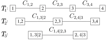
Figure 2: An example of 5-dim vine constructed with layouts {b,e,f,g,h}in Figure 2, and a valid choice of edges in it. For the sake of clarity, there is only one edge with the detail of its copula family and parameter.
Formally expressed, we have:
f(x1, x2, . . . , xd) =c(u1, u2, . . . , ud) d Y
i=1
fi(xi),
whereui=Fi(xi).
There are many families of parametric bivariate copula functions but only a few parametricd-variate ones. Among the latter, Gaussian and T copulas are quite flexible because depend on the correlation matrix of the transformed covari-ates. A better approach is to use bivariate copulas as building blocks for multivariate copulas. This solution was first pre-sented in (Joe 1996). Bedford and Cooke (2001) later devel-oped a more general factorization of multivariate densities and introduced regular vines.
Definition 3.1 (R-Vine ondvariables) A regular vine ond
variables consists ofd−1connected treesT1, ..., Td−1, that satisfy the following:
1. T1 consists of the node setN1 ={1, ..., d}, where each variable is represented by only one of the nodes; and the edge setE1, with each edge representing a copula that links two variables.
2. Fori= 2, . . . , d−1, the treeTiconsists of the node set Ni=Ei−1and the edge setEi
Tionly if their corresponding edges in TreeTi−1share a common node.
The regular vine copula(V,BV, θV)has density function
defined as:
c(u;V,BV, θV) = Y
Tk∈V Y
e∈Ek
cBe(ui(e)|D(e), uj(e)|D(e);θe)
whereBVis the set of bivariate copula families selected for
the VineVandθVthe corresponding parameters.
For the sake of clarity, let us consider 5 variables x1, . . . , x5, and that they have been already transformed
via their corresponding marginals intou1, . . . , u5, souk = fk(xk). According to definition 3.1, a Tree T1 will have
5 nodes and 4 edges. Therefore, its layout will necessarily be one out of those displayed in Figure 1(a–c). Each one of these layouts leads to many possible and different trees T1, depending on how variables are arranged in the layout.
For this example, let us assume that such an arrangement happens to be the one shown in the tree T1 of Figure 2,
in which it has been explicitly shown that the dependence (edge) betweenu3 andu5 is modeled with a Clayton
cop-ula, with parameterθ= 1.7. The layout of the next tree,T2
may, or may not be one out of Figure 1(d–e). It depends on whether it satisfies the third requirement. In this example, theT1layout in Figure 1(a) imposes the layout inT2to be
exclusively the one in Figure 1(d), resulting in the so called D-Vine. On the other hand, theT1layout in Figure 1(b)
al-lows both Figures 1(d) and 1(e) to be layouts forT2. When
arranging the variables in the layout, it is a good practice to write the actual variables, and not the edges of the prece-dent tree. Then, all variables shared in both nodes of an edge are turned into conditioning variables, and the remaining are conditioned. Eventually, the factorization of the copula den-sity is the product of all the nodes fromT2on. Thus, copula
density of the vine shown in Figure 2 is
c(u1, . . . , u5) =
c14c24c34c35c13|4c45|3c23|4c15|34c25|34c12|345
where the cij|k.. denotes the bi-variate copula density c Fi(xi|xk, ..),(Fj(xj|xk, ..)
.
4
Methodology
Model selection for vine is essentially a combinatorial prob-lem over a huge search space, which is hard to solve with heuristic approaches. Dissmann proposed a tree-by-tree ap-proach (Dissmann et al. 2013) , which selects maximum spanning trees at each level according to pairwise depen-dence. The problem with this locally greedy approach is that there is no guarantee that it will select a structure that is close to the optimal structure.
In this section, we describe in details our learning ap-proach for regular vine copula construction. In order to feed a vine configuration using a neural network based meta learning approach, we need to represent it in a compact way. Complexity arises since the construction of each level of tree depends on previous level’s tree. The generated vine also needs to satisfy the following desirable properties:
• Tree PropertyEach level in the vine should be a tree with no cycles.
• Dependence StructureThe layout of each level tree de-pends on its previous level’s tree.
• SparsityIn general, a sparse model where most of edges are independent copulas are preferred.
Next we compare two different representations for a regular vine model: Vector representation and RL representation.
Vector Representation
An intuitive way to embed a vine is to flatten all edges in the vine into a vector. Since the number of edges in the vine is fixed, the network can output a vector of edge indices. The representation proposed is depicted in Figure 3.
Let the set of edges in each tree beTk, the likelihood of the generated configuration can be computed as:
L= X Tk∈V
X
e∈Ek
logcBe(ui(e)|D(e), uj(e)|D(e);θe))
If the generated configuration contains a cycle at levelk, a penalty will be subtracted from the objective function. The penalty will decrease with the level, indicating that since later trees depend on early trees, violation in tree property in early levels will incur a larger penalty. Let the number of cycles at levelk∈ {1. . . K}beCk, thus the penalty due to violation of tree property can be computed as:
J1=
1
k K X
k=1
Ck
In practice, most variables are not correlated and the vines tend to be sparse. To avoid over-fitting, we favor smaller edges in the vine graph by adding a penalty termJ2, defined
as:
J2=
1 PK
k=1|Ek|
At each training iteration, we are maximizing the following objective function:
Jφ=L −λJ1+µJ2
whereλandµare hyper-parameters that can be tuned.
Reinforcement Learning Representation
Noise vector Z
FCNN
Ф
Ф
Ф
1 3
4 2
1
1,3
1,2 1,4
231 1
24 11 1
1 1
1 1 1
T1
T2
T3
T
node 1 in next tree
compute loss input x
1
T2
T3
1
1 2
2 3
Figure 3: A example of the vector representation of vine. The model takes in a random initial configuration vector and search for the best vector that maximizes the objective func-tion using a fully connected neural network (FCNN). The first element in the output vector (“Φ”) means that first node inT1is not connected, the second element (“1”) means that
second node inT1is connected to 1, etc. The layout on the
right shows how to take the output vector and assembles it into a regular vine.
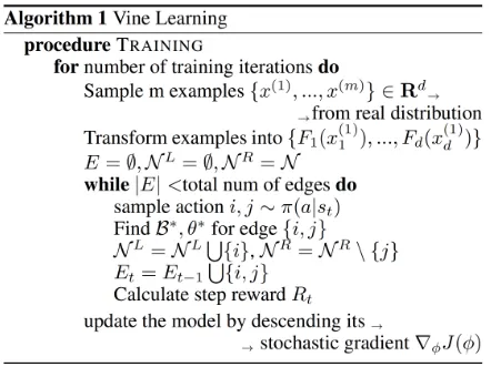
After we obtain the set of edges Ek for tree k, we re-peat the process for the next level of tree. The decision pro-cess can be defined as a fixed length sequence of actions of choosingE1, E2, E3, ...where|Ek|=d−k. For an untrun-cated vine withdvariables, the total number of edges adds up to d(d2−1). Motivated by recent developments in RL, we reformulate the problem in its syntax.
States Let et be the t-th edge added to the vine model, which consists of a pair of indexes(lt, rt). At step t, the states can be represented by the current set of edges in the vineEt, and the partitioned vertices setNtL andNtR. For-mallyst= (Et,NtL,NtR)is the state representation for the current vine at stept.
Actions The set of possible actions consists of all pairs of nodes that can be added to the current tree. FormallyAs= {(lt, rt) :iL∈ NL, iR∈ NR}.
Rewards The log likelihood of fitting a data pointxto the vinestat steptcan be decomposed into a set of trees and a set of independent nodes inNR
t that have not been added to the tree:
L(x, st) = X
e∈Et,e=(l,r)
log(cBe(ul|D(e), ur|D(e);θe)
+ X
i∈NR t
log(ui)
whereL(x, s0) =Pv∈Nlog(uv).
Then the incremental reward at stateStcan be defined as:
Rlikelihood(St) =L(x, st)− L(x, st−1)
=cBet(ult|D(et), urt|D(et);θet)
−log(urt)
whereetis the newly added edge to the vine.
As before, we add a penalty term to avoid over-fitting. Hence, the total reward is defined as:
R=Rlikelihood+λRpenalty
Policy Network LetPrbe the true underlying distribution, andPcbe the distribution of the network. Our goal is to learn a sequence of edges (pair of indices)Eof lengthN−1such that the following objective function is maximized:
Jφ=Eτ∼PcEx∼Pr "
L(x, s0) +
N−1
X
t=1
R(st) #
Letπφbe the stochastic policy defined implicitly by network Cφwith parametersφ. The policy gradient of the above ob-jective functionJφcan be computed as:
∇φJ(φ) =Eτ∼PcEx∼Pr "N−1
X
t=1
R(st)∇φlogπφ(τt|ˆst−1)
#
At each step, the policy network outputs a distribution over all possible actions, from which an action (edge) is sam-pled. Following standard practice, the expectation is approx-imated by sampling ndata points andmaction sequences per data point. Additionally, we use discounted reward and subtract a baseline term to reduce variance of gradients (Greensmith, Bartlett, and Baxter 2001).
Figure 4: Algorithm for learning vine structure
When constructing the Vine, a decision made in the first tree can affect to the nodes in deeper trees. Therefore, we cannot assure the markovian property, i.e. that the next state depends only of the current state and current decisions. A natural choice will be to adopt LSTM as a solution to this non-Markovian reinforcement learning tasks with long-term dependencies. Once the configuration is determined, we can find copula family and parameter for each edge following the method described in the following section.
Pair Copula Selection
1 3 2 4 1 3 2 4
1 3 2
4
Figure 5: A example of a training step for a 4-dim vine with RL formulation. The set of nodes is partitioned intoVL = {1,3}andVR ={2,4}. Node 1 inVLand node 2 inVRis sampled by the policy network and edge{1,2}is added to the vine.
Then we combine these three measurements in a hard-voting fashion to select a bivariate copula family according to the three-way check methods (Veeramachaneni, Cuesta-Infante, and O’Reilly 2015). The parameter is estimated according to its max likelihood fit after fitting the bivariate copula family. This provides us an approximated reward for adding an edge that guides us through the search space.
Sampling From A Vine
Figure 6: D-Vine of 4 variables.
After learning a vine model from the data, we can sam-ple synthetic data from it. Kurowicka and Cooke first pro-posed an algorithm to sample an arbitrary element from a regular vine, which they call the Edging Up Sampling Algorithm (Kurowicka and Cooke 2007). The sampling procedure requires a complete vine model of n nodes X1, X2, ..., Xn, and their corresponding marginal distribu-tionsF1, F2, ..., Fn. Considering the case where we have a D-Vine model with 4 nodes, shown in Figure 6. We start by sampling univariate distributionsu1, u2, u3, u4from
Uni-form Distribution over [0,1]. We randomly pick a node to start with, sayX2.
Then the first variablex2∼X2can be sampled as:
x2=F2−1(u2) (1)
After we have x2, we randomly pick a node connected to
X2. Suppose we pickX3, recall that the conditional density
f3|2can be written as:
f3|2(x3|x2) =f3(x3)c2,3(F2(x2), F3(x3)) (2)
=f3(x3)c2,3(u2, u3) (3)
=f3(x3)c3|2(u3) (4)
Thus,x3∼X3|X2can be sampled by:
x3=F3−1(C −1
3|2(u3)) (5)
whereC3|2can be obtained fromC2,3inT1by plugging in
sampled values ofu2.
Similarly, we pick a node that shares an edge withX3, say
X4. Thenx4∼X4|X2, X3can be sampled as:
x4=F4−1◦C −1 4|3◦C
−1
4|23(u4) (6)
Finallyx1∼X1|X2, X3, X4can be sampled as:
x1=F1−1◦C −1 1|4◦C
−1 1|34◦C
−1
1|234(u1) (7)
For a more general vine graph, we can use a modified Breadth First Search to traverse the tree and keep track of nodes that have already been sampled. The general proce-dure is described in Algorithm 4.
Figure 7: Algorithm for sampling from the learned vine
5
Experiments
Baselines and Experiment Setup
We compare our models with the tree-by-tree greedy ap-proach (Dissmann et al. 2013), which selects maximum spanning trees at each level according to pairwise depen-dence, as well as the bayesian approach (Gruber and Czado 2015). To test our approach, we used constructed examples. In this we construct vines manually, sample data from them and then use our learning approach to recreate the vine. We use two of the constructed examples defined in (Min and Czado 2010) and compare the results with both the greedy approach and the Bayesian approach. Second, we used three real data sets and compared the two approaches. The neural network used for creating vines for the vector representation is set-up as fully connected feed forward neural networks with two hidden layers. Each layer uses ReLU as activation function and the output layer is normalized by a softmax layer. The network for the reinforcement learning represen-tation is set up as LSTM. The algorithm is trained over 50 epochs in the experiments.
Constructed Examples
pre-specified regular vine. The fitting abilities of each model are measured by the ratio of log-likelihood of the estimated model and log-likelihood of the true underlying model. • Dense VineDense Vine is a 6-dim vine where all bivariate
copulas are non-independent. The bivariate families and thetas are listed in Table 6.
• Sparse Vine A 6-dim vine where all trees consisted of independent bivariate copulas except the first tree. In other words, the vine is truncated after the first level.
Table 1: Comparison of relative log-likelihood on con-structed examples. All results reported here are based on 100 independent trails.
Dense Sparse Dense T1 correct Dissmann relative loglik(%) 76.6 101.3 No Gruber relative loglik(%) 81.0 100.6 No Vector relative loglik(%) 80.3 99.8 No RL relative loglik(%) 84.2 100.2 Yes
In the dense vine example, the RL vine is the only model able to recover the correct first tree and also achieves the highest relative log-likelihood. In the sparse vine example, all four models achieve similar results, among which Diss-mann obtains the highest likelihood. As argued in (Min and Czado 2010), the higher likelihood in Dissmann is achieved at the expense of over-fitting. The two examples demonstrate the fitness of the model is improved by our model under dif-ferent scenarios. Moreover, for a 6-dimensional data set of size 500, the RL algorithm finishes in approximately 15 min-utes with a single GPU.
Real Data
In this section, we apply vine model to real data sets for the task of synthetic data generation. The three data sets that are picked are a binary classification problem, a multi-class classification problem and a regression problem. The batch size used is 64 for breast cancer dataset and 128 for the other two datasets. The three data sets used in experiments are: • Wisconsin Breast CancerDescribes 30 variables
com-puted from a digitized image of a fine needle aspirate (FNA) of a breast mass and a binary variable indicating if the mass is benign or malignant. This dataset includes 569 instances.
• Wine QualityThis dataset includes 11 physiochemical variables and a quality score between 0 and 10 for red (1599 instances) and white (4898 instances) variants of the Portuguese ”Vinho Verde” wine.
• CrimeThe communities and crime dataset includes 100 variables related to crimes ranging from socio-economic data to law enforcement data and an attribute to be pre-dicted (Per Capita Violent Crime) . This dataset has 1994 instances.
To evaluate the quality of the synthetic data, we first eval-uate its log likelihood. As shown in 2, synthetic data gener-ated from RL Vine achieves the highest log likelihood per instance in all three datasets.
Table 2: log-likelihood per instance truncated after third tree
Breast Cancer Wine Crime
Dissmann 0.79 0.033 0.26
Vector Rep 0.84 0.037 0.27
RL Vine 0.91 0.045 0.31
Besides log-likelihood, the quality of the generated syn-thetic data is also evaluated from a more practical perspec-tive. High quality synthetic datasets enable people to draw conclusions and make inferences as if they are working with a real data set. We first use both Dissmann’s algorithm and our proposed algorithms to learn copula vine models from a real data set. Later, we generate synthetic data from each model and train models for target variables on the synthetic training set as well as real training set, and use the real test-ing set to compute the correspondtest-ing evaluation metric (F1 score for classification and MSE for regression). For ease of computation, the learned vines are truncated after the third level, which means all pair copulas are assumed to be inde-pendent beyond the third level. All results reported are based on 10-fold cross-validation over different splits of training and testing set.
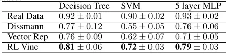
As shown in table 2 and table 3, synthetic data from RL Vine achieves highest F1 score and the results are compara-ble to real data. For regression data, tacompara-ble 4 demonstrates that synthetic data obtains lowest Mean Squared Error (MSE) among the models. The results shown demonstrate that our proposed model improve the overall model selection and is able to generate reliable synthetic data.
Table 3: F1 score of different end classifiers on breastcancer dataset
Decision Tree SVM 5 layer MLP Real Data 0.92±0.01 0.90±0.02 0.93±0.02
Dissmann 0.77±0.12 0.55±0.05 0.76±0.06
Vector Rep 0.76±0.09 0.62±0.07 0.71±0.05
RL Vine 0.81±0.06 0.72±0.03 0.79±0.03
Table 4: F1 score of different end classifiers on wine quality datset (averaged over 11 classes)
Decision Tree SVM 5 layer MLP Real Data 0.36±0.016 0.11±0.015 0.16±0.016
Dissmann 0.13±0.008 0.09±0.006 0.09±0.006
Vector Rep 0.15±0.011 0.07±0.004 0.08±0.005
RL Vine 0.21±0.006 0.09±0.006 0.11±0.008
Table 5: MSE error of different end classifiers on crime dataset
6
Conclusion
In this paper we presented a meta learning approach to cre-ate vine models for modeling high-dimensional data. Vine models allow for the creation of flexible structures using bivariate building blocks. However, to learn the best pos-sible model, one has to identify the best pospos-sible structure, which necessitates identifying the connections between the variables and selecting between the multiple bivariate cop-ulas for each pair in the structure. We formulated the prob-lem as a sequential decision making probprob-lem similar to rein-forcement learning, used long-short-term memory networks to simultaneously learn the structure and select the bivari-ate building blocks. We compared our results to the stbivari-ate of the art approaches and found that we achieve significantly better performance across multiple data sets. We also show that our approach can generate higher quality synthetic data that could be directly used to learn a machine learning model replacing the real data.
Acknowledgment
Dr. Cuesta-Infante is funded by the Spanish Gov-ernment Research Project TIN-2015-69542-C2-1-R (MINECO/FEDER) and the Banco de Santander grant for the Computer Vision and Image Processing Excellence Research Group (CVIP). Dr. Kalyan Veeramachaneni and Yi Sun acknowledge the generous funding provided by Accenture and National Science Foundation under the grant “CIF21 DIBBs: Building a Scalable Infrastructure for Data-Driven Discovery and Innovation in Education”, Award # 1443068.
7
Appendix
Experiment
Dense Copula Sparse Copula
C1,2 N(0.59) C1,2 N(0.41)
C2,3 C(0.71) C2,3 C(0.50)
C3,4 C180(0.80) C3,4 C180(0.50)
C3,5 N(-0.71) C3,5 N(-0.33)
C3,6 T(0.65,3) C3,6 T(0.49,5)
C1,3|2 G(0.75)
C2,4|3 N(0.41)
C2,5|3 C270(-0.60)
C2,6|3 N(-0.37)
C1,4|2,3 T(0.26,5)
C1,5|2,3 N(-0.26)
C1,6|2,3 C90(-0.56)
C4,6|1,2,3 N(0.13)
C5,6|1,2,3 C(0.20)
C5,6|1,2,3,4 G180(0.52)
Table 6: synthetic vine example. The pair copulas families used are: Gaussian(N) Clayton(C), Gumbel(G), Student’s T(T) and their corresponding rotations
References
Aas, K.; Czado, C.; Frigessi, A.; and Bakken, H. 2009. Pair-copula constructions of multiple dependence. Insurance: Mathematics and Economics44(2):182 – 198.
Alzantot, M.; Chakraborty, S.; and Srivastava, M. 2017. Sensegen: A deep learning architecture for synthetic sen-sor data generation. In2017 IEEE International Conference on Pervasive Computing and Communications Workshops, 188–193.
Bakker, B. 2001. Reinforcement Learning with Long Short-term Memory. In Proc. of the 14th Int. Conf. on Neural Information Processing Systems, NIPS’01.
Bedford, T., and Cooke, R. 2001. Probability density de-composition for conditionally dependent random variables modeled by vines. Annals of Mathematics and Artificial In-telligence32:245–268.
Carrera, D.; Santana, R.; and Lozano, J. A. 2016. Vine copula classifiers for the mind reading problem.Progress in Artificial Intelligence5(4):289–305.
Dissmann, J.; Brechmann, E.; Czado, C.; and Kurowicka, D. 2013. Selecting and estimating regular vine copula and ap-plication to financial returns. Computational Statistics and Data Analysis59:52–69.
Elidan, G. 2010. Copula bayesian networks. InAdvances in Neural Information Processing Systems 23, 559–567. Ganjali, M., and Baghfalaki, T. 2015. A Copula Approach to Joint Modeling of Longitudinal Measurements and Survival Times Using Monte Carlo Expectation-Maximization with Application to AIDS Studies.Journal of Biopharmaceutical Statistics25(5):1077–1099.
Goodfellow, I.; Bengio, Y.; and Courville, A. 2016. Deep Learning. The MIT Press.
Greensmith, E.; Bartlett, P. L.; and Baxter, J. 2001. Variance reduction techniques for gradient estimates in reinforcement learning. In Journal of Machine Learning Research, vol-ume 5, 1471–1530.
Gruber, L., and Czado, C. 2015. Sequential Bayesian Model Selection of Regular Vine Copulas. Bayesian Analy-sis10(4).
Gruber, L., and Czado, C. 2018. Bayesian model selection of regular vine copulas. Bayesian Analysis13(4).
Han, F.; Zhao, T.; and Liu, H. 2013. Coda: high dimen-sional copula discriminant analysis. J. Mach. Learn. Res.
14(1):629–671.
Hochreiter, S., and Schmidhuber, J. 1997. LONG SHORT-TERM MEMORY. InNeural Computation, 1735–1780. Joe, H. 1996. Families of m-variate distributions with given margins and m(m-1)/2 bivariate dependence parame-ters.Distributions with Fixed Marginals and Related Topics, IMS Lecture Notes - Monograpgh Series28:120–141. Jordan, M. I. 1999. Learning in Graphical Models. MIT Press.
Koller, D., and Friedman, N. 2009.Probabilistic Graphical Models: Principles and Techniques - Adaptive Computation and Machine Learning. The MIT Press.
Kurowicka, D., and Cooke, R. 2007. Sampling algorithms for generating joint uniform distributions using the vine-copula method. Computational Statistics & Data Analysis
51(6):2889–2906.
Kurowicka, D., and Joe, H. 2011. Dependence Modeling: Vine Copula Handbook. World Scientific Publishing Com-pany.
Li, H.; Xiong, L.; Zhang, L.; and Jiang, X. 2014. Dpsynthe-sizer: differentially private data synthesizer for privacy pre-serving data sharing. Proceedings of the VLDB Endowment
7(13):1677–1680.
Libes, D.; Lechevalier, D.; and Jain, S. 2017. Issues in syn-thetic data generation for advanced manufacturing. In2017 IEEE International Conference on Big Data (Big Data), 1746–1754.
Lopez-Paz, D.; Hernandez-Lobato, J.; and Ghahramani, Z. 2013. Gaussian process vine copulas for multivariate de-pendence. InJMLR 28(2): Proceedings of The 30th Interna-tional Conference on Machine Learning, 10–18. JMLR. MacKenzie, D., and Spears, T. 2014. ’The formula that killed Wall Street’: The Gaussian copula and modelling practices in investment banking. Social Studies of Science
44(3):393–417.
Min, A., and Czado, C. 2010. Bayesian inference for mul-tivariate copulas using pair-copula constructions.Journal of Financial Econometrics8(4):511–546.
Morales-Napoles, O. 2010. Dependence Modeling Vine Copula Handbook. World scientific. chapter Counting Vines, 189–218.
Muller, D., and Czado, C. 2018. Selection of sparse vine copulas in high dimensions with the lasso. Statistics and Computing29:269–287.
Nelsen, R. B. 2006. An introduction to copulas. Springer Series in Statistics, 2nd. edition.
Ratner, A. J.; Ehrenberg, H. R.; Hussain, Z.; Dunnmon, J.; and Christopher, R. 2017. Learning to Compose Domain-Specific Transformations for Data Augmentation. InProc. of Neural Information Processing Systems (NIPS) 2017, vol-ume 30, 3239–3249.
Sagduyu, Y.; Grushin, A.; and Shi, Y. 2018. Synthetic so-cial media data generation. IEEE Transactions on Compu-tational Social Systems1–16.
Soltana, G.; Sabetzadeh, M.; and Briand, L. 2017. Syn-thetic data generation for statistical testing. In 2017 32nd IEEE/ACM International Conference on Automated Soft-ware Engineering (ASE), 872–882.
Sutton, R. S., and Barto, A. G. 1998.Reinforcement learning - an introduction. MIT Press.
Veeramachaneni, K.; Cuesta-Infante, A.; and OReilly, U.-M. 2015. Copula Graphical Models for Wind Resource Estimation. In Proc. of the 24th Int. Joint Conference on Artificial Intelligence, IJCAI’15, 2646–2654.
Vinzamuri, B.; Li, Y.; and Reddy, C. K. 2014. Active learn-ing based survival regression for censored data. InProc. of the 23rd ACM Int. Conference on Information and Knowl-edge Management, CIKM’14, 241–250.
Wang, J., and Perez, L. 2017. The Effectiveness of Data Augmentation in Image Classification using Deep Learning. InArXiv.