The Thirty-Third AAAI Conference on Artificial Intelligence (AAAI-19)
Unsupervised Learning with Contrastive Latent Variable Models
Kristen A. Severson, Soumya Ghosh, Kenney Ng
Center for Computational Health and MIT-IBM Watson AI Lab, IBM Research, 75 Binney St. Cambridge, Massachusetts, 02142Abstract
In unsupervised learning, dimensionality reduction is an im-portant tool for data exploration and visualization. Because these aims are typically open-ended, it can be useful to frame the problem as looking for patterns that are enriched in one dataset relative to another. These pairs of datasets occur com-monly, for instance a population of interest vs. control or sig-nal vs. sigsig-nal free recordings. However, there are few meth-ods that work onsetsof data as opposed to data points or sequences. Here, we present a probabilistic model for dimen-sionality reduction to discover signal that is enriched in the
target dataset relative to thebackground dataset. The data in these sets do not need to be paired or grouped beyond set membership. By using a probabilistic model where some structure is shared amongst the two datasets and some is unique to the target dataset, we are able to recover interesting structure in the latent space of the target dataset. The method also has the advantages of a probabilistic model, namely that it allows for the incorporation of prior information, handles missing data, and can be generalized to different distribu-tional assumptions. We describe several possible variations of the model and demonstrate the application of the technique to de-noising, feature selection, and subgroup discovery set-tings.
Introduction
In unsupervised learning, the goal is often to learn what is unique or interesting about a dataset. Given the subjective nature of this question, it can be useful to frame the problem in the context of what signal is enriched in one dataset, re-ferred to as thetarget, relative to a second dataset, referred to as thebackground. An example of this is an exploration of a heterogeneous disease population, such as patients with Parkinson’s disease. The interesting sources of variation are those that are unique to the disease population. However, it is likely that some sources of variation are unrelated to the disease state, for instance variation due to aging. This is dif-ficult to assess without a baseline population, therefore, it is useful to contrast the disease population with a population of healthy controls. Suchcontrastive analysiscan discover nui-sance variation that is common amongst the two populations
Copyright c2019, Association for the Advancement of Artificial Intelligence (www.aaai.org). All rights reserved.
Supplemental information is available at https://arxiv.org/
and is uninteresting for the problem while highlighting vari-ation unique to the disease populvari-ation enabling downstream applications such as subgroup discovery.
Despite this natural setting for unsupervised learning, most techniques address individual data points, sequences, or paired data points. Few techniques generalize to the con-trastive scenario where we have sets of data but no obvious correspondence between their members. Yet, there are many cases where datasets that can be used in a comparative set-ting arise naturally: control vs. study populations, pre- and post-intervention groups, and signal vs. signal free groups (Abid et al. 2018). Each of these settings has possible nui-sance variation, for example, population level variation, ef-fects unrelated to intervention, and sensor noise variation.
The recently published contrastive principal component approach (cPCA) (Abid et al. 2018) is one example of a technique that can be used for sets of data. cPCA builds on principal component analysis (PCA) (Hotelling 1933), a di-mensionality reduction technique which projects data into a lower dimensional space while minimizing the squared loss. PCA and other dimensionality reduction techniques are pop-ular because they allow high-dimensional data to be visual-ized while removing noise. cPCA seeks to find a projection to a lower dimensional space that discovers variation that is enriched in one dataset as compared to another by applying PCA to the empirical covariance matrix
C= 1
n
n
X
i=1
xixTi −α
1
m
m
X
j=1
yjyTj (1)
where {xi} are the observations of interest, {yj} are the comparison data, andαis a tuning parameter. The choice of
αis a trade-off between maximizing the retained variance of the target set and minimizing the retained variance of the background set.
noise distributions, model and feature selection can be per-formed through sparsity promoting prior distributions, and the model can more easily be incorporated into larger prob-abilistic systems in a principled manner. Through this paper, we advance the state-of-the-art in several ways. First, we de-velop latent variable models capable of contrastive analy-sis. We then demonstrate the generality of our framework by demonstrating how robust and sparse contrastive variants can be developed, learned and how automatic model selec-tion can be performed. We also develop contrastive variants of the variational autoencoder, a deep generative model, and demonstrate its utility in modeling the density of noisy data. Finally, we vet our proposed models through extensive ex-periments on real world scientific data to demonstrate the utility of the proposed framework.
Contrastive Latent Variable Models
To achieve the aim of discovering patterns that are enriched in one dataset relative to another, we propose a latent vari-able model where some structure is shared across the two datasets and some structure is unique to the target dataset. Given a target dataset {xi}ni=1 and a background dataset{yj}m
j=1, the model is specified
xi =Szi+Wti+µx+i, i= 1. . . n yj =Szj+µy+j, j = 1. . . m
(2)
wherexi,yj ∈ Rd are the observed data,zi,zj ∈ Rk and ti ∈ Rtare the latent variables,S∈ Rd×k andW ∈Rd×t
are the corresponding factor loadings,µx,µy ∈Rdare the
dataset-specific means andi,j∈Rdare the noise. In
gen-eral, we do not expect the number of samples in the two datasets to be the same, i.e.n 6= m. Furthermore, there is no special relationship between the samplesiandjin equa-tion 2. The primary variables of interest are{ti}n
i=1, which
are the lower dimensional representation that is unique to the target dataset.
Gaussian likelihood and priors
To provide intuition into why eqn. 2 meets our goal of capturing patterns enriched in the target with respect to the background, we consider the case where the noise fol-lows isotropic Gaussian distributions,i ∼ N(0, σ2Id)and j ∼ N(0, σ2Id)and the latent variables are modeled using standard Gaussian distributions
xi|zi,ti∼ N(Szi+Wti+µx, σ2Id) yj|zj ∼ N(Szj+µy, σ
2I
d)
zi∼ N(0,Ik), zj∼ N(0,Ik), ti∼ N(0,It), (3)
whereN(µ,Σ)is a multivariate normal distribution param-eterized by meanµand covarianceΣandIddenotes ad×d identity matrix. The resulting marginal distributions for the observed data are
xi∼ N(µx,WW
T+SST+σ2Id)
yj∼ N(µy,SS T+σ2I
d).
(4)
The covariance structure for the target data is additive and contains a term (SST) that is shared with the background
data and a term that is unique to the target data (WWT). This constructions allows the factor loading W to model the structure unique to the target. The model closely mir-rors probabilistic PCA (PPCA) (Tipping and Bishop 1999; Roweis 1998) and is exactly PPCA applied to the combined datasets when the target factor loading dimensionalityt is zero. Similarly, this model is exactly PPCA applied to only the target dataset when the shared factor loading dimen-sionalitykis zero. Expectation-maximization (EM) (Demp-ster, Laird, and Rubin 1977) can be used to solve for the model parameters. Because EM requires conjugacy, most model formulations will not be solved this way. However, we present a summary of the EM steps to provide an intu-ition about the model. To provide interpretable equations in the below description, we consider the case where the factor loading matricesWandSare orthogonal.
The model parameters areS,W,µx,µy,σ2and the latent variables arezi,zj,ti. The lower bound of the likelihood is
L=
n
X
i=1
Ep(zi,ti|xi)[lnp(zi,ti,xi)]+
m
X
j=1
Ep(zj|yj)[lnp(zj,yj)]
(5)
The M-step maximizes the lower bound of the likelihood with respect to the parameters. The update step for the shared factor loading is
˜
S=(B+ (I−WR−1WT)T)S
(σ2I+M−1ST(B+T)S)−1 (6)
whereBis the sample covariance of the background data,T is the sample covariance of the target data,M=σ2Ik+STS, andR=σ2I
t+WTW. The update step for the target factor loading is
˜
W= ((I−SM−1S)TW)(σ2I+R−1WTTW)−1 (7)
Details on the derivation can be found in the supplemen-tal information. It is useful to recall that the orthogonal projection onto the range space of a matrix A is given byP = A(ATA)−1AT and the orthogonal projection onto the nullspace of A is given by I − P. In eqn. 7, I −
SM−1Scan be expanded using the definition ofMtoI−
S(σ2Ik +STS)−1ST. Similarly, in eqn. 6, I−WQ−1WT can be expanded using the definition ofQtoI−W(σ2I
The update steps can also be compared to the PPCA up-dates. For the factor loading matrixW, the update step is:
˜
W=TW(σ2I+R−1WTTW)−1 (8)
which is the same as eqn. 7, except for the projection term.
Beyond Gaussian Models
The assumptions of Gaussianity are not necessary for re-covering latent structure that enriches desired patterns in the target dataset. We can more generally express the proposed model as:
p(D,{zi,ti}ni=1,{zj}mj=1; Θ) =
p(Θ)
n
Y
i=1
p(xi|zi,ti;W,S,µx, σ2)p(zi)p(ti)
m
Y
j=1
p(yj|zj;S,µy, σ
2)p(z
j),
(9)
where D = {{xi}n i=1,{yj}
m
j=1} and Θ =
{W,S,µx,µy, σ2}. The primary modeling decisions
are to choose the appropriate likelihoods and priors on the loading matrices. The particular choices are governed by the application and domain specific knowledge.
However, this flexibility comes at a price: the poste-rior distributionsp(ti,zi,zj|D)are no longer guaranteed to be tractable. Consequently, the EM algorithm sketched in the previous section is no longer available and instead, we use variational inference (Wainwright and Jordan 2008). In summary, the intractable posteriors are approximated with tractable surrogatesq(ti|λti)q(zi|λzi)q(zj|λzj)and diver-gence KL(q||p)is minimized with respect to the variational parametersλ={{λzi, λti}n
i=1,{λzj} m
j=1}. This is
equiva-lent to maximizing the lower bound of the marginal likeli-hood,
p(D; Θ)≥ L(λ,Θ)
=X
i
Eq(zi;λzi)q(ti;λti)[lnp(xi|zi,ti; Θ\{µy})]
−KL(q(zi;λzi)||p(zi))−KL(q(ti;λti)||p(ti))
+X
j
Eq(zj;λzj)[lnp(yj|zj; Θ\{µx,θx})]
−KL(q(zj;λzj)||p(zj)) +lnp(Θ)
(10) where Θ\{·} implies the parameters in Θ except the
pa-rameters denoted in the set. Depending on the choice of
q and p the expectations required for computing L(λ,Θ)
may themselves be intractable. We use recently proposed black box techniques (Ranganath, Gerrish, and Blei 2014; Kingma and Welling 2014; Rezende, Mohamed, and Wier-stra 2014; Titsias and L´azaro-Gredilla 2014) to sidestep this additional complication. In particular, we approximate the intractable expectations in L(Θ, λ) with unbiased Monte-Carlo estimates,L˜(Θ, λ). Because the latent variables of in-terest are continuous, we are able to use reparameterization gradients (Kingma and Welling 2014; Rezende, Mohamed, and Wierstra 2014) to differentiate through the sampling
process and obtain low variance estimates of∇λ,ΘL(Θ, λ),
∇λ,ΘL˜(Θ, λ). Using the noisy but unbiased gradients,
opti-mization can proceed using a stochastic gradient ascent vari-ant, e.g. ADAM (Kingma and Ba 2014). In our experiments we use Edward (Tran et al. 2016), a library for probabilis-tic modeling, to implement these inference strategies for the proposed models. We sketch the pseudocode for variational learning in Algorithm 1.
Algorithm 1Pseudocode
1: Input Model p(D; Θ), variational approximations
q({zi, ti}ni=1,{zj}mj=1|λ)
2: Output: OptimizedΘand variational parametersλ
3: InitializeλandΘ. 4: repeat
5: Use reparameterization trick to compute unbiased es-timates of the gradients of the objective in Eqn. 10,
∇λ,ΘL˜(λ,Θ)
6: Update λ(l+1) ← ADAM(λ(l),∇
λL˜(λ,Θ)),
Θ(l+1)←ADAM(Θ(l),∇
ΘL˜(λ,Θ))
7: untilconvergence
Finally, we note that the black box inference framework does not restrict us to point estimates ofΘ. As we will il-lustrate in the next section, it is possible to infer variational distributions overΘby specifying an appropriate approxi-mationq(Θ|λΘ).
cLVM Variants
We refer to the base structure of the model as provided in eqn. 9 as a contrastive latent variable model, cLVM. As pre-viously noted, different choices for the distributions in eqn. 9 can be made to address the specific challenges of the appli-cation. Several models are introduced here and are summa-rized in Table 1.
Sparse cLVM One application-specific problem is feature selection. In unsupervised learning, there is often a sec-ondary goal of learning a subset of measurements that are of interest which is motivated by improved interpretability. This is especially important when the observed data is very high-dimensional. For instance, many biological assays re-sult in datasets that have tens of thousands of measurements such as SNP and RNA-Seq data. During data exploration, discovering a subset of these measurements that is impor-tant to the target population can help guide further analysis. To learn a latent representation that is only a function of a subset of the observed dimensions, certain rows of the target factor loading, W, must be zero. The observed data corre-sponding to the zero rows in Wthen have no contribution to the latent representationt. Because there is no restriction onS, a sparsity requirement forWdoes not imply that the corresponding observation is zero.
Model name Prior Likelihood Variational Approximation
cLVM – Gaussian –
Sparse cLVM p(W) =
Qd
i=1N(Wi:|ρi, τ)
C+(ρi|0,1)C+(τ|0, bg)
Gaussian
q(W) =N(·,·)
q(lnρ) =N(·,·)
q(lnτ) =N(·,·)
cLVM with
model selection p(S) =
Qd−1
i=1N(S:j|0, αj)IG(αj|a, b) Gaussian
q(S) =N(·,·)
q(lnα) =N(·,·)
Robust cLVM p(σ2) =IG(a, b) Student’s t q(lnσ2) =N(·,·)
cVAE – Gaussian parameterizedby neural network q(zi,ti) =N(gµ(·), gσ(·))
Table 1: Summary of the model variants. For all of the models in the table, the latent variables{zi,ti}ni=1,{zj}mj=1are modeled
as standard Gaussians and the variational distributions are also Gaussian, unless otherwise noted. The model choice depends on the application. The various models are not mutually exclusive and may also be combined.
logp(W) ∝ r(W), wherer(·)is the penalty function. For feature selection, a group sparsity penalty (Yuan and Lin 2007) could be used. The rows ofW∈Rd×tare penalized:
r(W) =ρ
d
X
i=1
√
pikWi:k2 (11)
where Wi: is the ith row of W. This functional form is
known to lead to sparsity at the group level, i.e. all mem-bers of a group are zero or non-zero. For increasing values ofρ, the target factor loading matrix has a larger number of zero-valued rows.
Sparsity inducing priors such as the automatic relevance determination (ARD) (Bishop 1999a; Virtanen et al. 2011; Klami, Virtanen, and Kaski 2013) or global-local shrinkage priors such as the horseshoe (Carvalho, Polson, and Scott 2009; 2010) can also be easily incorporated into the frame-work ˙Using the horseshoe prior as an example, theithrow of Wis modeled,
Wi:|ρi, τ ∼ N(0, ρ2iτ
2It)
ρi∼C+(0,1), τ ∼C+(0, bg)
(12)
wherea ∼ C+(0, b)is the half-Cauchy distribution with
densityp(a|b) = 2
πb(1 + a2
b2)fora >0. The horseshoe prior
is useful for subset selection because it has heavy tails and an infinite spike at zero. Further discussion can be found in the supplemental information. For both the prior and regu-larization formulations,groupsof rows inWcould also be used instead of single rows if such a grouping exists.
cLVM with Automatic Model Selection The ARD prior is more typically applied to the columns of a factor loading matrix. This use allows for automatic selection of the di-mension of the matrix. This could also be done in the cLVM model. Although both latent spaces can have any dimension less than d, which must be selected, we generally recom-mend setting the target dimension to two for visualization purposes. To select the dimension of the shared space, the percent variance explained can be analyzed or a prior, such as the ARD prior can be used. The columns ofSare modeled S:j|αj∼ N(0, αjId), αj∼IG(a0, b0). (13)
The ARD prior has been shown to be effective at model se-lection for PPCA models (Bishop 1999b).
Robust cLVM Another application-specific goal may be to systematically handle outliers in the dataset. Similar to PPCA, the cLVM model is sensitive to outliers and can pro-duce poor results if outliers are not addressed. It may be possible to remove outliers from the dataset, however this is typically a manual process that requires domain exper-tise and an understanding of the process that generated the data. A more general approach to handling outliers uses a heavy-tailed distribution to describe the data. One approach for constructing heavy tailed distributions is through scale mixtures of Gaussians (West 1987). Consider,
σ2∼IG(a, b). (14)
The resulting marginal distribution of the observed data is
p(xi|µ, a, b) =
d
Y
k=1
Z ∞
0
N(xik|µ, σ2)IG(σ2|a, b)dσ2
=
d
Y
k=1
St(xik|µ, ν= 2a, λ= a
b)
(15)
where St indicates a Student’s t-distribution (Archambeau, Delannay, and Verleysen 2006). The larger probability mass in the tails of the Student’s t-distribution, as compared to the normal distribution, allows the model to be more robust to outliers.
Beyond Linear Models
Contrastive Variational Autoencoders Thus far we have only considered models that linearly map latent variablesz andtto the observed space. The linearity constraint can be relaxed, and doing so leads to powerful generative models capable of accounting for nuisance variance.
xi =fθs(zi) +fθt(ti) +i, i= 1. . . n yj=fθs(zj) +j, j= 1. . . m,
wherei ∼ N(0, σ2),j ∼ N(0, σ2), andfθs,fθt rep-resent non-linear transformations parameterized by neural networks. The latent variables are modeled using standard Gaussian distributions, as before. Observe that similar to the linear case (eqn. 2) the target and background data share the projectionfθs while the target retains a private projection
fθt. This construction forcesfθs to model commonalities between the target and background data while allowingfθt to capture structure unique to the target.
This model can be learned by maximizing the lower bound to the marginal likelihood p(D|Θ),
Θ ={θs, θt, µx, µy, σ2}, analogously to eqn. 10. However, a large amount of data is typically required to learn such a non-linear model well. Moreover, since the number of latent variables proliferate with increasing data, it is computationally more efficient to amortize the cost of inferring the latent variables through inference networks shared between the data instances. In particular, we parametrize the variational posteriors qλt(zi,ti|xi) =
N(zi|gλµt(xi), gλσt(xi))N(ti|g µ λt(xi), g
σ
λt(xi) and
q;λs(zj|yj) = N(zj|g µ λs(yj), g
σ
λs(yj)), where λt and
λsare inference network parameters. Unlike eqn. 10 where the variational parameters grow with the number of data instances, the variational parameters λtandλs do not. λt is shared amongst the target instances while λs is shared between the background examples. This is an example of amortized variational inference (Dayan et al. 1995; Gershman and Goodman 2014). Finally, learning proceeds by maximizing the evidence lower bound,
p(D; Θ)≥ L(Θ, λs, λt)
=X
i
Eqλt(zi,ti|xi)[lnp(xi|zi,ti; Θ\{µy})]
−KL(qλt(zi,ti|xi)||p(zi)p(ti))
+X
j
Eqλs(zj|yj)[lnp(yj|zj; Θ\{µx,θx})]
−KL(qλs(zj|yj)||p(zj)) +lnp(Θ), (17) with respect to Θandλs,λt. The KL terms are available to us in closed form, however the expectation terms are in-tractable and we again resort to Monte Carlo approximations and re-parameterized gradients to enable stochastic gradient ascent. We refer to this combination of the non-linear model and the amortized variational inference scheme as the con-trastive variational auto encoder (cVAE).
Related Work
There are many techniques for dimensionality reduction, e.g. (Hotelling 1933; van der Maaten and Hinton 2008; Cox and Cox 2008). This review focuses on dimensionality techniques that use sets of data and/or address issues related to nuisance variation. Canonical correlation analysis (CCA) (Hotelling 1936) and its probabilistic variant (PCCA) (Bach and Jordan 2005) use two (or more) sets of data, however re-quires that samples are paired views (or higher dimensional sets of views) of the same sample. For instance perhaps sev-eral tests are run on a single patient and therefore the tests are linked via the patient identity. In CCA, the number of
samples in the sets must be equal,n=m, however the di-mensionality of each sample does not need to be the same. Damianou, Lawrence, and Ek proposed a nonlinear exten-sion of PCCA where the mappings are sampled from a Gaus-sian process. The resulting model is a multi-view extension of GP-LVM (Lawrence 2005), but still requires linking the samples across datasets.
In this work, we propose addressing nuisance variation in the dataset by introducing a structure to the latent repre-sentation. Schulam and Saria investigate a similar idea with respect to sharing representations across different parts of the full data. In their work, a hierarchical model for disease trajectory is proposed where some of the model coefficients are shared across subsets of the data, e.g. total population and individual. This idea has also been proposed for the unsupervised analysis of time series data (Hsu, Zhang, and Glass 2017; Li and Mandt 2018). Data samples are assumed to have a latent representation that can be partitioned into static and dynamic contributions. None of these works have considered a contrastive setting. There has also been work in addressing explicit sources of nuisance variation. Louizos et al. explores a setting where certain variables within the dataset are a priori identified as nuisance and the remain-ing variables contribute to the latent representation. The ob-served data is modeledx∼pθ(z,s)wheresare the observed nuisance variables.
Experiments
Contrastive latent variable models have applications in sub-group discovery, feature selection, and de-noising, each of which is demonstrated here leveraging different modeling choices. We use examples from Abid et al. to highlight the similarities and differences between the two approaches. The results of cLVM as applied to synthetic datasets can be found in the supplemental information.
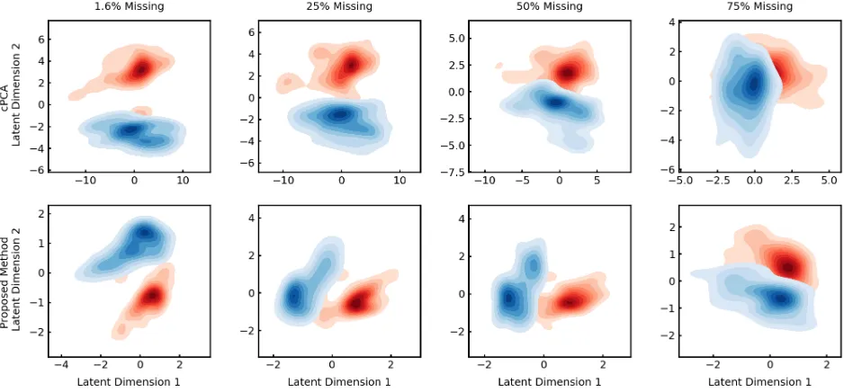
Subgroup Discovery for Incomplete Data
Figure 1: cLVM is robust to missing data. Density plots of the subgroups revealed in the target latent representation of the mice protein expression data. Red and blue points are the control and trisomic mice samples, respectively. The rows use cPCA and robust cLVM to learn the latent representation, respectively. Each column uses a different level of missing data, starting with the leftmost column containing the natural level of missing data. PCA is unable to perform subgroup discovery (see supplemental information) and robust cLVM is better able to perform subgroup discovery in the presence of missing data.
missing data. cPCA does not have natural handling for miss-ing data therefore mean imputation was used to first fill-in. PCA is unable to recover the structure in the dataset (see supplemental information for results). Both cPCA and ro-bust cLVM find the subsets, however, the proposed method is better able to discover the subgroups as the amount of missing data increases.
Subgroup Discovery for High Dimensional Data
To highlight the use of cLVM for subgroup discovery in high-dimensional data, we use a dataset of single cell RNA-Seq measurements (Zheng et al. 2017). The target dataset consists of expression levels from 7,898 samples of bone marrow mononuclear cells before and after stem cell trans-plant from a leukemia patient. The background contains ex-pression levels from 1,985 samples from a healthy individ-ual. Pre-processing of the data reduces the dimensionality from 32,738 to 500 (Zheng et al. 2017; Abid et al. 2018). Given the size of the data to explore, it is useful in this set-ting to use an ARD prior to automatically select the dimen-sionality of the shared latent space. The target latent space is set to two and an IG(10−3,10−3) prior is used for the
columns of the shared factor loading. Fig. 2a shows the re-sulting latent representation, which is able to discover the subgroups, whereas PCA is not (see supplemental informa-tion). Fig. 2b compares the percent of variance explained in the ranked columns as compared to the cLVM model without model selection. The model with ARD uses over 100 fewer columns in the shared factor loading matrix and avoids an analysis to manually select the dimension.
Automatic Feature Selection using Sparse cLVM
The third example uses a dataset, referred to as mHealth, that contains 23 measurements of body motion and vi-tal signs from four types of signals (Banos et al. 2014; 2015). The participants in the study complete a variety of ac-tivities. The target data is composed of the unknown classes of cycling and squatting and the background data is com-posed of the subjects lying still. In this application, we demonstrate feature selection by learning a latent represen-tation that both separates the two activities and uses only a subset of the signals. A group sparsity penalty is used, as described in the methodology, on the target factor loading. The target dimension is two, the shared dimension is twenty, andρis 400.ρis selected by varying its value and inspect-ing the latent representation. The latent representation us-ing regularization is shown in Fig. 2c. The two classes are clearly separated. Fig. 2d shows the row-wise norms of the target factor loading. The last six dimensions, corresponding to the magnetometer readings, are all zero which indicates that the magnetometer measurements are not important for differentiating the two classes and can be excluded from fur-ther analysis.
De-noised Generative Modeling using cVAE
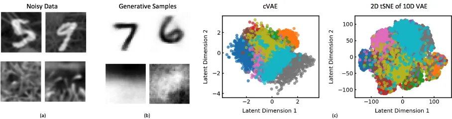
Finally, to demonstrate the utility of cVAE, we consider a dataset of corrupted images (see Fig. 3a). This dataset was created by overlaying a randomly selected set of 30,000
Figure 2: cLVM variants allow for model and feature selection. (a) Subgroups revealed in the target latent representation for the RNA-Seq dataset using the model selection cLVM variant. (b) The percent variance explained by the ordered columns of the shared factor loading for LVM with and without ARD (model selection). The ARD model has over 100 fewer non-zero columns in the shared factor loading. (c) Subgroups revealed in the target latent representation for the mHealth dataset using sparse cLVM. (d) The norms of the rows of the target factor loading for sparse LVM where the different colors correspond to different sensor types. The six dimensions with zero-valued norms correspond to magnetometer readings.
Figure 3: cVAE recovers meaningful structure from noisy data. (a) Samples of the target noisy images of digits on grass and background grass images. (b) Generative samples of the de-noised target (top row) and background (bottom row) which are enabled by the cVAE structure. Note there is no correspondence between the samples in (a) and (b). (c) The 2D cVAE projection and a 2D tSNE projection of a VAE with 10 dimensional space. The colors represent different digits.
a cVAE with a two-dimensional target latent space and an eight-dimensional shared space. We use fully connected en-coder and deen-coder networks with two hidden layers with
128 and 256 hidden units employing rectified-linear non-linearities. For the cVAE, both the target and shared de-coders θs andθt use identical architectures. We compare against a standard variational autoencoder with an identical architecture and employ a latent dimensionality of ten, to match the combined dimensionality of the shared and target spaces of the contrastive variant. Fig. 3c presents the results of this experiment. The latent projections for the cVAE clus-ter according to the digit labels. VAE on the other hand con-founds the digits with the background and fails to recover meaningful latent projections. Moreover, cVAE allows us to selectively generate samples from the target or the back-ground space, Fig. 3b. The samples from the target space capture the digits, while the background samples capture the coarse texture seen in the grass images. Additional compar-isons with a VAE using a two dimensional latent space is available in the supplemental.
Conclusions
Dimensionality reduction methods are important tools for unsupervised data exploration and visualization. We pro-pose a probabilistic model for improved visualization when the goal is to learn structure in one dataset that is enriched as compared to another. The latent variable model’s core characteristic is that it shares some structure across the two datasets and maintains unique structure for the dataset of interest. The resulting cLVM model is demonstrated using robust, sparse, and nonlinear variations. The method is well-suited to scenarios where there is a control dataset, which is common in scientific and industrial applications.
References
Abid, A.; Zhang, M. J.; Bagaria, V. K.; and Zou, J. 2018. Ex-ploring patterns enriched in a dataset with contrastive principal component analysis. Nature Communications9:2134.
Bach, F. R., and Jordan, M. I. 2005. A probabilistic interpretation of canonical correlation analysis. Technical report, University of California, Berkeley.
Banos, O.; Garcia, R.; Holgado, J. A.; Damas, M.; Pomares, H.; Rojas, I.; Saez, A.; and Villalonga, C. 2014. mhealthdroid: A novel framework for agile development of mobile health applica-tions. In6th International Work-conference on Ambient Assisted Living and Daily Activities, 91–98. Springer.
Banos, O.; Villaonga, C.; Rafael, G.; Saez, A.; Damas, M.; Holgado-Terriza, J. A.; Lee, S.; Pomares, H.; and Rojas, I. 2015. Design, implementation, and validation of a novel open framework for agile development of mobile health applications.
BioMedical Engineering Online14:1–20.
Bishop, C. M. 1999a. Variational principal components. In
ICANN, 509–514. IEE.
Bishop, C. M. 1999b. Bayesian PCA. InNIPS, 382–388.
Carvalho, C. M.; Polson, N. G.; and Scott, J. G. 2009. Handing sparsity via the horseshoe. InAISTATS, 73–80. JMLR.
Carvalho, C. M.; Polson, N. G.; and Scott, J. G. 2010. The horseshoe estimator for sparse signals.Biometrika97:465–480. Cox, M. A. A., and Cox, T. F. 2008. Multidimensional scaling. InHandbook of Data Visualizations. Springer. 315–347. Damianou, A.; Lawrence, N. D.; and Ek, C. H. 2016. Multi-view learning as a nonparametric nonlinear inter-battery factor analysis.arXiv preprint arXiv:1604.04939.
Dayan, P.; Hinton, G. E.; Neal, R. M.; and Zemel, R. S. 1995. The helmholtz machine.Neural computation7(5):889–904. Dempster, A. P.; Laird, N. M.; and Rubin, D. B. 1977. Maximum likelihood from incomplete data via the em algorithm.Journal of the Royal Statistics Society. Series B (Methodological)39:1–38. Gershman, S., and Goodman, N. 2014. Amortized inference in probabilistic reasoning. InProceedings of the Annual Meeting of the Cognitive Science Society, volume 36.
Higuera, C.; Gardiner, K. J.; and Cios, K. J. 2015. Self-organizing feature maps identify proteins critical to learning in a mouse model of down syndrome.PLOS ONE10:e0129126. Hotelling, H. 1933. Analysis of a complex of statistical variables into principal components. Journal of Educational Psychology
24:417.
Hotelling, H. 1936. Relations between two sets of variables.
Biometrika28:321–377.
Hsu, W.-N.; Zhang, Y.; and Glass, J. 2017. Unsupervised learn-ing of disentangled and interpretable representations from se-quential data. InNIPS, 1878–1889.
Kingma, D. P., and Ba, J. 2014. Adam: A method for stochastic optimization.arXiv preprint arXiv:1412.6980.
Kingma, D. P., and Welling, M. 2014. Stochastic gradient vb and the variational auto-encoder. InICLR.
Klami, A.; Virtanen, S.; and Kaski, S. 2013. Bayesian canoni-cal correlation analysis. Journal of Machine Learning Research
14:965–1003.
Lawrence, N. 2005. Probabilistic non-linear principal compo-nent analysis with Gaussian process latent variable models. Jour-nal of Machine Learning Research6:1783–1816.
LeCun, Y.; Bottou, L.; Bengio, Y.; and Haffner, P. 1998. Gradient-based learning applied to document recognition. In
Proceedings of the IEEE, 2278–2324.
Li, Y., and Mandt, S. 2018. Disentangled sequential autoencoder. InICML, 5656–5665. PMLR.
Louizos, C.; Swersky, K.; Li, Y.; Welling, M.; and Zemel, R. 2016. The variational fair autoencoder. InICLR.
Ranganath, R.; Gerrish, S.; and Blei, D. M. 2014. Black box variational inference. InAISTATS, 814–822.
Rezende, D. J.; Mohamed, S.; and Wierstra, D. 2014. Stochastic backpropogration and approximate inference in deep generative models. InICML, 1278–1286. PMLR.
Roweis, S. T. 1998. EM algorithms for PCA and SPCA. In
NIPS, 626–632.
Russakovsky, O.; Deng, J.; Su, H.; Krause, J.; Satheesh, S.; Ma, S.; Huang, Z.; Karpathy, A.; Khosla, A.; Bernstein, M.; Berg, A. C.; and Li, F.-F. 2015. Imagenet large scale visual recognition challenge. International Journal of Computer Vision115:211– 252.
Schulam, P., and Saria, S. 2015. A framework for individualizing of disease trajectories by exploiting multi-resolution structure. In
NIPS, 748–756.
Tipping, M. E., and Bishop, C. M. 1999. Probabilistic princi-pal component analysis.Journal of the Royal Statistical Society, Series B61:611–622.
Titsias, M., and L´azaro-Gredilla, M. 2014. Doubly stochastic variational Bayes for non-conjugate inference. InICML, 1971– 1979. PMLR.
Tran, D.; Kucukelbir, A.; Dieng, A. B.; Rudolph, M.; Liang, D.; and Blei, D. M. 2016. Edward: A library for probabilistic model-ing, inference, and criticism.arXiv preprint arXiv:1610.09787. van der Maaten, L., and Hinton, G. 2008. Visualizing data using t-SNE.Journal of Machine Learning Research9:2579–2605. Virtanen, S.; Jia, J.; Klami, A.; and Darrell, T. 2011. Factorized multi-modal topic model. InProceedings of the Conference on Uncertainty in Artificial Intelligence, 843–851. ACM.
Wainwright, M. J., and Jordan, M. I. 2008. Graphical models, exponential families, and variational inference.Foundations and TrendsR in Machine Learning1(1–2):1–305.
West, M. 1987. On scale mixtures of normal distributions.
Biometrika74:646–648.
Yuan, M., and Lin, Y. 2007. Model selection and estimation in regression with grouped variables. Journal of the Royal Statisti-cal Society, Series B68:49–67.