The Thirty-Third AAAI Conference on Artificial Intelligence (AAAI-19)
Sentence-Wise Smooth
Regularization for Sequence to Sequence Learning
Chengyue Gong,
†∗Xu Tan,
§Di He,
†Tao Qin
§ †Peking University§Microsoft Research
§{xuta,taoqin}@microsoft.com,†{cygong,di he}@pku.edu.cn
Abstract
Maximum-likelihood estimation (MLE) is widely used in se-quence to sese-quence tasks for model training. It uniformly treats the generation/prediction of each target token as multi-class multi-classification, and yields non-smooth prediction proba-bilities: in a target sequence, some tokens are predicted with small probabilities while other tokens are with large proba-bilities. According to our empirical study, we find that the non-smoothness of the probabilities results in low quality of generated sequences. In this paper, we propose a sentence-wise regularization method which aims to output smooth predic-tion probabilities for all the tokens in the target sequence. Our proposed method can automatically adjust the weights and gradients of each token in one sentence to ensure the pre-dictions in a sequence uniformly well. Experiments on three neural machine translation tasks and one text summarization task show that our method outperforms conventional MLE loss on all these tasks and achieves promising BLEU scores on WMT14 English-German and WMT17 Chinese-English translation task.
1
Introduction
Sequence to sequence learning has achieved great success in many natural language processing (NLP) tasks such as machine translation (Bahdanau, Cho, and Bengio 2014; Cho et al. 2014; Wu et al. 2016; Vaswani et al. 2017; Gehring et al. 2017; He et al. 2018; Song et al. 2018; Shen et al. 2018), text summarization (Rush et al. 2015; Shen et al. 2016) and dialog systems (Serban et al. 2016). The most popular model architecture for sequence to sequence learning is the encoder-decoder framework, which learns a probabilistic mapping
P(y|x)from a source sequencexto a target sequencey. During training, maximum-likelihood estimation (MLE) is widely used to learn the model parameters. Sincey = {y1, y2,· · ·, yn}is a sequence of tokens, by decomposing
P(y|x)using the chain rule, MLE becomes to minimize the average of the negative log probabilities of individual target tokens−1
n
Pn
i=1logP(yi|y<i,x;θ)over all(x,y)pairs in
training data, whereθis the model parameter. While MLE training objective sounds reasonable in general, it has sev-eral potential issues in the context of sequence to sequence
∗
The work was conducted when the first author was an intern at Microsoft.
Copyright c2019, Association for the Advancement of Artificial Intelligence (www.aaai.org). All rights reserved.
tasks, such as exposure bias (Wiseman and Rush 2016; Wu et al. 2018; Guo et al. 2019), loss-evaluation mismatch (Wiseman and Rush 2016; Vijayakumar et al. 2016), and myopic bias (He et al. 2017).
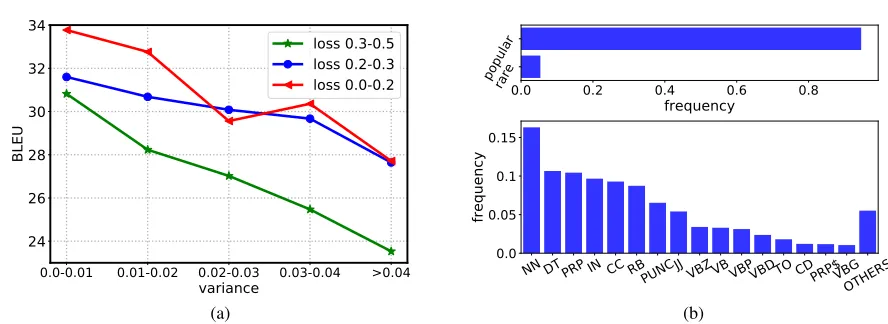
In this paper, we investigate the MLE loss for sequence to sequence tasks from an optimization and algorithmic per-spective. According to our empirical study, we find that for a well-trained model, the probabilities of individual tokens (i.e., per-token probabilities) in the target sequence for a given source sequence sometimes vary dramatically across time steps. We conduct an analysis on WMT14 English-German validation set to explore the relationship between the smoothness1of probabilities and BLEU scores, as shown
in Figure 1(a). As can be seen, for source-target pairs with same/similar MLE loss, the smoother the per-token probabil-ities are, the higher BLEU score is. Intuitively speaking, for source-target sequence pairs with the same/similar MLE loss, the sequence pair with non-smooth probabilities indicates that it has more small and large per-token probabilities. First, if the probability of certain target token is relatively low, the model is likely to make a wrong prediction for this token and thus generates a bad sequence during inference. Second, if the probability of certain target token is extremely large, i.e., larger than 0.9, which is enough to ensure correct prediction, there is no need to continue optimizing this token and it’s bet-ter to leave the efforts of the model to other low-probability tokens.
Besides, we wonder where the non-smooth problem comes from and then study the components of tokens with low probability in the train set. As is well-known, rare words are hard to learn (Gong et al. 2018) and low probabilities may just come from rare words. However, as shown in Figure 1(b), we find that nearly 6% of low-probability tokens are rare words, and this ratio almost equals to the ratio of rare words in the whole dataset, which demonstrates low-probability tokens do not prefer rare words more than popular words.2We further partition the low-probability tokens into different POS tags and find that the major part are nouns, determiners, pronouns,
1
Here we simply use variance to represent the smoothness for clearness and simplicity at the beginning of the paper. The formal definition of the smoothness obeys the definition in Section 3.2.
2
0.0-0.01 0.01-0.02 0.02-0.03 0.03-0.04 >0.04
variance
24
26
28
30
32
34
BLEU
loss 0.3-0.5
loss 0.2-0.3
loss 0.0-0.2
(a)
0.0 0.2 0.4 0.6 0.8
frequency
rare popular
NN DT PRP IN CC RBPUNCJJ VBZVBVBPVBDTO CDPRP$VBGOTHERS
0.0 0.05 0.1 0.15
frequency
(b)
Figure 1: (a): The variance of per-token probabilities negatively correlates with BLEU scores. We choose the translation sentences from WMT14 English→German validation set based on a well-trained Transformer model (experimental details are in Section 4). We partition the sentence pairs into three groups according to the MLE loss: 0-0.2, 0.2-0.3, 0.3-0.5, and divide the sentence pairs in each group into 5 buckets according to the variance of token probabilities: 0-0.01, 0.01-0.02, 0.02-0.03, 0.03-0.04, ¿0.04. Different colors represent different MLE loss groups. (b): The components of the tokens with low probability in IWSLT14 German→English training set based on a well-trained Transformer model. We analyze the components from the perspective of popular/rare words as well as different POS tags. More details about these analyses in (a) and (b) can be found in supplementary materials (part A).
conjunctions and punctuations,3 and ratio of conjunctions
and pronouns in low-probability tokens are higher than the ratio in the whole dataset. More detailed discussions are listed in supplementary materials (part A). From these analyses, we find the low-probability tokens are not mainly caused by rare words and thus the non-smooth probabilities cannot be addressed effectively by the conventional methods tackling rare words (Luong and Manning 2016; Li, Zhang, and Zong 2016).
Inspired by the above observations, in this work, we aim to learn a sequence generation model which can output smooth per-token probabilities across time steps. We first design two principles (Prediction Saturation and Wooden Barrel) for a loss function to ensure the smoothness of per-token probabil-ities. We then design a sentence-level smooth regularization term adding to the MLE loss to guide the training process. We show that our proposed loss satisfies both principles while the conventional MLE loss does not. The designed regularization term aims at reducing the variance of per-token probabili-ties across time steps and make those probabiliprobabili-ties smoother. When there are tokens with both large and small probabilities in a sequence, the regularizer actually sacrifices the loss of to-kens with large target probability only a little (which usually does not hurt the training and inference much), focuses on optimizing losses for the tokens of small probabilities (which may bring advantages), and leads to sequences with smoother per-token probabilities and consequently better performance. To demonstrate the effectiveness of our proposed loss, we conduct experiments on three machine translation tasks and one text summarization task. The results show that our de-signed loss indeed leads to smooth per-token probabilities
3
We use Natural Language Toolkit to do POS tag: https://www.nltk.org/.
and consequently better performance: Our method outper-forms baseline methods on all the tasks and sets new records on all the three NMT tasks.
2
Maximum-Likelihood Estimation
In this section, we briefly describe how MLE works in se-quence to sese-quence learning. Denote(x,y)as a source-target sequence pair, wherexis a sequence from the source domain andy is a sequence from the target domain. Sequence to sequence learning aims to model the conditional probabil-ityP(y|x;θ), whereθis the model parameter. The widely adopted MLE lossLM LE(x,y;θ)defined on a sequence pair
(x,y)is as follows.
LM LE(x,y;θ) =−logP(y|x;θ)
=−
n
X
i=1
logP(yi|y<i,x;θ),
(1)
wherey<iis the sequence of the preceding tokens before
positioniandnis the length of the target sequence. For sim-plicity, we denoteP(yi|y<i,x;θ)aspi. By applying length
normalization, we have
LM LE(x,y;θ) =−
1 n
n
X
i=1
logpi, (2)
wherepiis a function of(x,y, θ). We call the probabilities
(p1, p2,· · ·, pn)as theprobability sequence, which is further
denoted asp. The sub-sequence(pi,· · ·, pj)from time step
itoj is denoted aspi:j. In general, the loss is a function
of the probability sequence and we denote it as L(p) or
3
Our Method
In this section, we first introduce two principles that a loss function should satisfy (while MLE can not) to ensure smooth per-token probabilities. We then propose a sentence-wise smooth regularization term, and show that equipped with the regularization term, the MLE loss satisfies these principles.
3.1
Principles
Clearly, to generate smoothp, we need to reduce the vari-ance and difference of per-token probabilities. To achieve this, intuitively, a loss function should guide the optimization procedure to pay less attention to tokens of large probabili-ties and more attention to tokens of small probabiliprobabili-ties. We specify two principles regarding this as follows.
Prediction Saturation (PS)When the prediction of a token in the target sequence is good enough and much better than other tokens, further improving this token brings no more gain or even negative gain to the overall loss. We call such a principle theprediction saturationprinciple.
Wooden Barrel (WB)As well known, the capacity of a bar-rel is determined not by the longest wooden bars, but by the shortest. If the prediction probability of a token is small while its adjacent tokens are relatively large, it becomes the barrier during inference and makes the probability sequence non-smooth. We hope the efforts that the optimization algorithm puts to this token positively correlates with the gap between the probability of the token and that of its neighbors. We call such a principle thewooden barrelprinciple.
The above two principles are mathematically characterized as follows.
Definition 1 (PS Principle). Suppose (β, ) is a pair of positive constants. We say an objective function L(p1, p2,· · ·, pn) is(β, )-saturated, if∀i, p0i ≥ pi ≥ β
andmax(pi−1, pi+1)≤β−, the following inequality holds:
L(· · ·, pi,· · ·)≤L(· · ·, p0i,· · ·).
This principle means that if the prediction of a token is good enough, i.e., its probability is larger than a threshold
β, and its adjacent tokens are not well optimized, i.e., their probabilities are smaller thanβ−, further improving this good enough token (e.g., pushingpito a large valuep0i) does
not lead to the decrease of the loss.
Definition 2 (WB Principle). Denote i∗ = argmini(p1,· · · , pn) . We say an objective
func-tion L(p1, p2,· · ·, pn) is γ-focused, if for any
p0i∗+1 > pi∗+1 ≥γ+pi∗ andp0i∗−1 > pi∗−1 ≥γ+pi∗,
the following inequality holds:|∂L(···,pi∗ −1,pi∗,pi∗+1,···)
∂pi∗ |< |∂L(···,p
0
i∗ −1,pi∗,p0i∗+1,···)
∂pi∗ |.
This principle suggests that if the prediction probability of a token is small and its adjacent tokens are of large probabil-ities, the absolute value of the gradient of the loss function with respect to this token increases when enlarging the prob-ability of its adjacent tokens. Such a principle guarantees that the optimization will focus on tokens that are not well optimized.
Note that several previous works actually satisfy the PS principle, although they do not explicitly define the
princi-ple. For example, curriculum learning and self-paced learn-ing (Bengio et al. 2009; Pentina, Sharmanska, and Lampert 2015) tend to pay less attention to easy training samples ac-cording to handcraft rules or model outputs, but they fail to satisfy the WB principle.
As the MLE loss is the sum of log probabilities of tokens across positions and is a strictly decreasing function ofpi,
it is easy to check that the MLE loss does not satisfy the above two principles and thus will not lead to smooth per-token probabilities. The proof is provided in supplementary materials (part B).
3.2
The Proposed Loss
Our new loss is the combination of the MLE loss and a smooth regularization term.
For a sequence with lengthn, we can obtainn−k+1 subse-quences using a sliding window with sizek. We first consider the smoothness within each subsequence and then compute the overall smoothness for the whole sequence. In detail, for each sub-sequence(pi,· · · , pi+k−1), we define its
smooth-nessrias the L2-norm of the distance between adjacent
prob-abilities in the subsequence:ri=
q
Pk−2
j=0(pi+j−pi+j+1)2.
If the distance between adjacent probabilities is large,riwill
be large. We further introduce a weight factor wi for the
smoothness of the subsequence in each sliding window:
wi= 1−min(pi,· · ·, pi+k−1). (3)
Intuitively,wiup weights the subsequence with small
proba-bilities, and down weights subsequence with large probabili-ties.
Then our new loss is designed as follow:
Lsmo=
1 n(−
n
X
i=1
log pi+λ n−k+1
X
i=1
wiri), (4)
where the first term is the MLE loss, the second term is the proposed smooth regularization term, which is a weighted average over the smoothness of the subsequence in each sliding window, andλis a hyper-parameter controlling the trade-off between the MLE loss and the regularization term.
3.3
Analysis
In this subsection, we show that our proposed loss Lsmo
satisfies the two principles in Section 3.1.
Theorem 1. Lsmohas the following properties: Whenk= 2,
Lsmo is(β,λβ1 +β−1)-saturated. Whenk > 2,Lsmo is
(β,q 1
2√kβλ)-saturated.
Proof. The theorem is equivalent to show∂Lsmo
∂pi ≥0when max(pi−1, pi+1)≤β−andpi≥β.
Fork= 2case, Wheni∗>0, we have∂Lsmo
∂pi =
1 n(−
1 pi+ λ(2−pi−1−pi+1)). Whenpi≥βandmax(pi−1, pi+1)≤
β − = 1− 1
2λβ, we have ∂Lsmo
∂pi ≥ −
1 β +λ
1 λβ = 0.
ThenLsmois(β,2λβ1 +β−1)-saturated. Wheni∗= 0, we
have ∂Lsmo
∂pi =
1 n(−
1
pi+1≤β−= 1−λβ1 , we have ∂L∂psmoi ≥ −1β+λλβ1 = 0.
ThenLsmois(β,λβ1 +β−1)-saturated.
For generalk, we have:
∂Lsmo
∂pi
= 1 n(−
1 pi
+λ
i
X
j=i−k+1
wj(2pi−pi+1−pi−1)rj−1). (5)
Asrj≤
√
kand=q 1
2√kβλ, we have:
∂Lsmo ∂pi = 1 n[ 1 pi +λ i X
j=i−k+1
wj(2pi−pi+1−pi−1)r−j1]
≥ 1
n[− 1 β+λ
i
X
j=i−k+1
(1−β+)(2pi−pi+1−pi−1)rj−1]
≥ 1
n[− 1
β+λk(1−β+)2
r
1 k].
(6)
It is easy to check that(1−β+)≥ √
k
2kλβ. Therefore, ∂Lsmo
∂pi ≥0. The theorem follows.
We provide a more intuitive explanation of the principle. The corollary below shows how the loss function works when the prediction probability is≥0.5.
Corollary 1. Lsmois(12,λ1−12)-saturated whenk= 2, and
is(12,q 1
λ√k)-saturated whenk >2.
Corollary 1 shows a special case whenβ = 0.5. When
pi ≥β = 0.5, the token will be correctly predicted, since
the probability 0.5 is larger than the sum of the remaining probabilities in the softmax output. In such a situation, when
k= 2, once the prediction probability of a nearby token is smaller than 1λ−1
2, the loss will not continue optimizingpi
to a large value.
Theorem 2. Lsmohas the following properties: Whenk= 2,
Lsmois0-focused. Whenk >2,Lsmois0.193-focused.
Proof. DenoteL0smo=Lsmo(· · · , p0i∗−1, pi∗, p0i∗+1,· · ·).
Fork = 2 case, wheni∗ ≥ k, by definition, we have
∂L0smo ∂pi∗ =
1 n[−
1
pi∗ +λ(2pi
∗−p0i∗−1−pi0∗+1)]<n1[−p1
i∗ +
λ(2pi∗−pi∗−1−pi∗+1)] = ∂Lsmo
∂pi∗ , and
∂Lsmo
∂pi∗ <0. when k= 2, i∗< k, since2pi∗−p0i∗+1−1<2pi∗−pi∗+1−1
and2pi∗−p0i∗−1−1<2pi∗−pi∗−1−1(ifi∗−1exists), we
have∂L
0 smo
∂pi∗ <
∂Lsmo
∂pi∗ <0. Therefore, the loss is0-focused.
For generalk, similar to the proof of Theorem 1, we have
∂Lsmo
∂pi∗ =
1 n[−
1 pi∗+λ
Pi∗
j=i∗−k+1{−rj+ (1−pi∗)(2pi∗− pi∗+1 − pi∗−1)rj−1}]. Denote x = pi∗+1 − pi∗, y = pi∗−1 −pi∗, a = rj2 −x2 −y2, c = 1−pi∗, we have rj−(1−pi∗)(2pi∗−pi∗+1−pi∗−1)r−1
j =c x+y
√
x2+y2+a + p
x2+y2+a = f(x). Without lose of any generality,
we treat this term as a function of x. Then, it is suffi-cient to show f(x)is strictly monotone increasing when
pi∗±1 ≥ γ+pi∗. Aspi∗±1 ≥ 0.193 +pi∗, we havey > 0.193candx >0.193c. Using Cauchy-Schwarz Inequality,
we havef0(x) ≥ (x3+y2x−cyx+cy2)
(x2+y2+a)−32
≥ (33 √
cx4y4−cyx)
(x2+y2+a)−32
≥
(3cyx√30.1932−cyx)
(x2+y2+a)−32
>0. Therefore,∂L
0 smo
∂pi∗ <
∂Lsmo
∂pi∗ .
The theorem follows.
Theorem 1 and Theorem 2 together theoretically study our proposed lossLsmo. In the next section, we will empirically
show thatLsmocan ensure smooth per-token probabilities
and improve the performance of sequence to sequence learn-ing.
4
Experiments
We test our method on three translation tasks as well as a text summarization task. We first introduce the datasets and experiment settings. Then we report the results of our method and compare it with several baselines. We also conduct some analyses to investigate how our proposed loss works. In this section, we mark our proposed loss asSmoothfor simplicity.
4.1
Datasets
WMT14 English-German TranslationFollowing the setup in (Luong et al. 2015; Gehring et al. 2017; Vaswani et al. 2017), the training set of this task consists of 4.5M sentence pairs. Source and target sentences are encoded by 37K shared sub-word types based on byte-pair encoding (BPE) (Sen-nrich, Haddow, and Birch 2015). We use the concatenation of newstest2012 and newstest2013 as the validation set and newstest2014 as the test set.
WMT17 Chinese-English Translation We filter the full dataset of 24M bilingual sentence pairs by removing duplica-tions and get 19M sentence pairs for training. The source and target sentences are encoded using 40K and 37K BPE tokens. We report the results on the official newstest2017 test set and use newsdev2017 as the validation set.
IWSLT14 German-English TranslationThis dataset con-tains 160K training sentence pairs and 7K validation sentence pairs following (Cettolo et al. 2014). Sentences are encoded using BPE with a shared vocabulary of about 37K tokens. We use the concatenation of dev2010, tst2010, tst2011 and tst2011 as the test set, which is widely adopted in (Huang et al. 2017; Bahdanau et al. 2016; Tan et al. 2019).
Text SummarizationWe use the English Gigaword Fifth Edition (Graff et al. 2003) corpus for text summarization, which contains 10M news articles with the corresponding headlines. We follow (Rush et al. 2015; Shen et al. 2016) to filter the article-headline pairs and get roughly 3.8M pairs for training and 190K pairs for validation. We test our method on the widely used Gigaword test set with 2K article-title pairs (Shen et al. 2016; Suzuki and Nagata 2017).
4.2
Implementation Details
We choose Transformer (Vaswani et al. 2017) as our basic model and use tensor2tensor (Vaswani et al. 2018), which is an encoder-decoder structure purely based on at-tention and achieves state-of-the-art accuracy on several se-quence to sese-quence learning tasks.
For WMT14 English-German task, we choose both
Dataset Setting Method BLEU
En→De
Transformer Base
MLE 27.30*
Curriculum 27.41
Smooth 28.32
Transformer Big
MLE 28.40*
Curriculum 28.22
Smooth 29.01
Zh→En Transformer Big
MLE 24.30
Curriculum 24.06
Smooth 25.05
De→En Transformer Small
MLE 32.20
Curriculum 31.97
Smooth 33.47
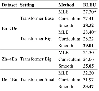
Table 1: BLEU scores on the three NMT tasks. Our method is denoted as “Smooth” and the curriculum learning method is denoted as “Curriculum”. BLEU scores marked with * are from (Vaswani et al. 2017).
Dataset Method BLEU
En→De
Local Attention (Luong et al. 2015) 20.90 ConvS2S (Gehring et al. 2017) 25.16 Transformer Base (Vaswani et al. 2017) 27.30 Transformer Big (Vaswani et al. 2017) 28.40 Transformer Base+Smooth 28.32 Transformer Big+Smooth 29.01
Zh→En
SougoKnowing (Wang et al. 2017) 24.00 xmunmt (Tan et al. 2017) 23.40
Transformer+Smooth 25.05
De→En
Actor-critic (Bahdanau et al. 2016) 28.53 CNN-a (Gehring et al. 2016) 30.04 Dual transfer learning (Wang et al. 2018) 32.35
Transformer+Smooth 33.47
Table 2: Comparison with previous works.
(Vaswani et al. 2017). Both the configurations have a 6-layer encoder and a 6-layer decoder, with 512-dimensional and 1024-dimensional hidden representations, respectively. For WMT17 Chinese-English task, we usetransformer big con-sidering the large scale of the training set. For IWSLT14 German-English task, we choosetransformer smallwith a 2-layer encoder/decoder and 256-dimensional hidden rep-resentations. For the text summarization task, we choose
transformer smallwith a 4-layer encoder/decoder and
256-dimensional hidden representations. Unless otherwise stated, we keep all other hyper-parameters the same as (Vaswani et al. 2017). Unless otherwise stated, in all our experiments, the sliding windowkof subsequences in our loss is set to4and
λis set to0.6according to the validation performance.
We choose Adam optimizer withβ1 = 0.9,β2 = 0.98,
ε= 10−9. We follow the learning rate schedule in (Vaswani
et al. 2017). During inference, for WMT14 English-German and WMT17 Chinese-English tasks, we use beam search with beam size6and length penalty1.0(Shen et al. 2016). For IWSLT14 German-English task and the text summarization task, we set beam size to6and length penalty to1.1. These hyper-parameters are chosen after experimentation on the development set.
Our method is to train the Transformer model by min-imizing the loss defined in Equation 4. We compare our method with the MLE loss based method. We also compare with a token-level curriculum learning (Bengio et al. 2009; Pentina, Sharmanska, and Lampert 2015) method. The strat-egy for selecting examples in this curriculum learning is as follows. As the training process goes on, this baseline tends to focus on hard tokens: It ignores target tokens with probabil-ities larger than0.85, and only updates its model using tokens with probabilities smaller than0.85. All the three methods use the same model configurations for fair comparisons.
We use the ROUGE F1 score (Lin 2004)4to measure the text summarization quality. For fair comparisons, we use the tokenized case-sensitive BLEU (Papineni et al. 2002)5 to measure the translation quality for WMT14 En→De, scare-BLEU6for WMT17 Zh→En, and tokenized case-insensitive BLEU for IWSLT14 De→En. For both the two metrics, the bigger the better. We use the validation performance to choose a goodλand setkto 4.
4.3
Results of Machine Translation
We compare our method with the corresponding MLE and curriculum learning baselines, and then with the results re-ported in several previous works. We denote WMT14 English-German task as En→De, WMT17 Chinese-English task as Zh→En and IWSLT14 German-English task as De→En.
The BLEU scores are listed in Table 1. As can be seen, the curriculum learning method does not significantly out-perform the MLE baseline. This result suggests that only focusing on hard instances and not meeting the WB principle (instead of smoothing per-token probabilities) is not enough for sequence to sequence learning. For WMT14 En→De task, our method with thetransformer basemodel reaches 28.32 BLEU score, i.e., 1.02 BLEU score improvement over the MLE loss in (Vaswani et al. 2017). We also achieve 0.61 BLEU score improvement from 28.40 to 29.01 on the
transformer bigmodel. For WMT17 Zh→En and IWSLT14
De→En tasks, our method improves the BLEU score from 24.30 to 25.05 and 32.20 to 33.47, respectively.
We further list the numbers reported in previous works on the three tasks in Table 2. Note that those works use dif-ferent model structures, including LSTM (Hochreiter and Schmidhuber 1997), CNN (Gehring et al. 2017), and Trans-former (Vaswani et al. 2017). For WMT14 En→De task, our
4Calculated by https://github.com/pltrdy/rouge 5
https://github.com/moses-smt/mosesdecoder/blob/master/ scripts/ generic/multi-bleu.perl
6
method achieves 29.01 BLEU score, outperforming the best number formally published so far and setting a new record on this dataset. For WMT17 Zh→En task, our method beats the champion7of WMT17 Zh→En challenge by 1.05 BLEU
score. For IWSLT14 De→En task, our method also achieves 1.12 BLEU score improvement.
For all above tasks, we have done significant test, and the improvements are significant where all p-value<0.05. The improvements on the three tasks demonstrate the effective-ness of our proposed sentence-wise smooth regularization for sequence to sequence learning.
0-0.1 0.1-0.2 0.2-0.3 0.3-0.4 0.4-0.5 0.5-0.6 0.6-0.7 0.7-0.8 0.8-0.9 0.9-1.0
probability 0.0
0.1 0.2 0.3 0.4 0.5
frequency
Train MLE Train Smooth Valid MLE Valid Smooth
Figure 2: Comparison of the per-token probability frequency between our proposed method and the MLE baseline in
trans-former baseon WMT14 English-German train and validation
set. The red lines show the results on the training set and the blue lines show the results on the validation set.
4.4
Method Analysis
In this subsection, we conduct some analyses to better under-stand our proposed method.
Distribution of per-token probabilities We first analyze how the distribution of the per-token probabilities changes when applying our proposed method. We conduct this study on WMT14 English-German training and validation set. We divide the probability interval [0,1] into ten buckets. For both our proposed loss and the MLE baseline, we calculate the frequency of the per-token probabilities in each bucket, as shown in Figure 2. From the figure, we can see that our method reduces the frequency of both small (smaller than 0.5 in the figure) and very big (larger than 0.9 in the figure) probabilities while greatly increases the frequency of the probabilities located in[0.7,0.9]. This demonstrates that our method indeed makes the per-token probabilities smoother. We further study the changes in loss and list them in sup-plementary materials (part C). Besides, we have analyzed the variance changes and found that the variance becomes smaller after applying our method on IWSLT14 De-En test set. The sentences originally with high variance get lower variance and higher BLEU score improvements. Specifically,
7
We choose the best single model for comparison, as the best result is obtained by combining multiple models (http://matrix.statmt.org/matrix/systems list/1878).
we divided sentences into 5 groups according to their variance in the MLE training: the group with highest variance gets 1.47 BLEU score improvements on average in our method, while the sentence with lowest variance has 0.35 BLEU score improvements.
λ 0.4 0.6 0.8 1.0 2.0
BLEU 33.19 33.47 33.42 33.39 33.26
Table 3: The BLEU scores with respect to differentλon IWSLT De→En task.
Hyper-parameter λ is used to control the effect of our smooth regularization. In previous experiments, we use the validation performance to choose a goodλ. Here we study howλimpacts the performance of our method. We train a group of models with differentλon IWSLT De→En task. The results are listed in Table 3. It can be seen that too small or too bigλwill hurt the performance of our method. This is consistent with Theorem 1 and 2 that too smallλcannot ensure the regularization effect, while too largeλ overempha-sizes the smoothness. We also study the influence of another hyper-parameter: the sliding windowk, and list the results in supplementary materials (part D).
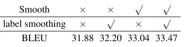
Label Smoothing(Szegedy et al. 2015; Vaswani et al. 2017) is related to our work in the sense that it makes the true label less confident in training. While applying the cross-entropy loss to a classification task, it is usually expected to output probability 1 for true labels and 0 for the others. However, as the true labels are often the aggregated results of multi-ple annotators, there may be some disagreements among the annotators. Thus, label smoothing relaxes the target probabil-ities of true labels, e.g., assigning probability 0.9 instead of 1 and allocating 0.1 to other labels. Actually, the open-source code of Transformer has already implemented label smooth-ing, and the Transformer based methods (including both the baseline method and our method) adopt this technique in our experiments.
It seems that label smoothing can also prevent the prob-ability from being too large, and therefore we do an abla-tion study to compare our method with label smoothing. As shown in Table 4, only adding label smoothing improves 0.32 BLEU score, while adding our method alone can im-prove 1.16 BLEU score. Further adding our method to label smoothing achieves 1.27 BLEU score improvement.
Case StudyIn this subsection, we present several translation cases to demonstrate how our proposed method improves the sequence generation accuracy, as shown in Table 5. We have following observations.
Smooth × × √ √
label smoothing × √ × √
BLEU 31.88 32.20 33.04 33.47
Source ich habe ihnen ein beispiel mitgebracht von dem nordamerikanischen stamm der nootka-indianer .
Reference i brought along an example of the north american tribe of the nootka indians .
MLE i’ve brought you an example of the north american tribe .
Smooth i brought you an example of the north american tribe of the nootka indian .
Source also wir haben vorne die augen und jetzt denken sie , wir sehen von vorne nach hinten .
Reference so we have our eyes at the front and now you think we see from front to back .
MLE so we’ve got the front , and now you’re thinking , we’re looking forward from the back .
Smooth so we’ve got the eyes forward , and now you think , we’re going to look back from the front .
Source da konnten dann die besucher in den raum reingehen, sich auf diesen stuhl setzen, sich diesen helm aufsetzen.
Reference visitors could go into the room , sit down on this chair , and put on this helmet .
MLE and then the visitor in the room could put themselves on this chair , put it on that helmet .
Smooth then the visitor could go into the room , sit down on that chair , put that helmet on .
Table 5: Examples of the translation results by our proposed method (”Smooth”) and the MLE baseline (”MLE”) on IWSLT14 De→En test set.
First, our method helps the model to generate more accu-rate and fluent sequence. For example, in the second case, our method catches the information ‘look from front to back’, which is misunderstood by the MLE baseline. In the third case, the MLE baseline fails to recognize ‘put on helmet’ and ‘sit on chair’, which are correctly translated by our method.
Second, rare words, prepositions and conjunctions, usually skipped/ignored by the MLE baseline, are well captured by our method. For example, the phrases ‘of the nootka indian’ and ‘have brought’ in the first case and the token ‘eyes’ in the second case are generated by our method but missed by the baseline method. These tokens are usually of low probabilities predicted by the baseline model and are likely to be neglected in the beam search process.
Model R-1 R-2 R-L
RNN MRT(Shen et al. 2016) 36.54 16.59 33.44
WFE(Suzuki and Nagata 2017) 36.30 17.31 33.88 ConvS2S(Gehring et al. 2017) 35.88 17.48 33.29
Transformer 35.34 16.44 32.71
Transformer+Curriculum 35.61 16.36 32.78
Transformer+Smooth 36.32 17.17 33.54
Table 6: The ROUGE-1/2/L scores for different methods on the text summarization task.
4.5
Results of Text Summarization
Table 6 shows the results of the text summarization task. Com-pared with the MLE loss, our method improves the ROUGE-1/2/L by 1.0, 0.7, 0.9 points. Besides, our method also outper-forms the curriculum learning baseline. Compared with other previous works including minimize risk training (Shen et al.
2016; 2015), WFE (Suzuki and Nagata 2017) that cutting off redundant repeating, our method achieves comparable results. These methods have different motivations from ours. There-fore, note that these works are orthogonal to our method and we expect to obtain more improvements by combining with these methods.
5
Conclusion and Future Work
In this paper, we observed that in sequence to sequence learning, sentences with non-smooth probabilities are usually of low quality. We design a new loss with a sentence-wise smooth regularization term to solve this problem. Experimen-tal results show that our method outperforms the conventional MLE loss and achieves state-of-the-art BLEU scores on the three machine translation tasks. There are many directions to explore in the future. First, we focused on machine transla-tion and text summarizatransla-tion in this work. We will apply our method to more sequence generation tasks, such as image captioning and question answering. Second, we will inves-tigate if there exist better methods to ensure the probability sequence to be smooth. Third, the smoothness of token proba-bilities is motivated from empirical observations in this work. It is interesting to study the smoothness of loss from a theoret-ical perspective, e.g., why a smooth loss function is preferred, and what it brings to the learning method.
References
Bahdanau, D.; Brakel, P.; Xu, K.; Goyal, A.; Lowe, R.; Pineau, J.; Courville, A.; and Bengio, Y. 2016. An actor-critic algorithm for sequence prediction. arXiv preprint
arXiv:1607.07086.
Bahdanau, D.; Cho, K.; and Bengio, Y. 2014. Neural machine translation by jointly learning to align and translate. arXiv
Bengio, Y.; Louradour, J.; Collobert, R.; and Weston, J. 2009. Curriculum learning. InICML, 41–48. ACM.
Cettolo, M.; Niehues, J.; St¨uker, S.; Bentivogli, L.; and Fed-erico, M. 2014. Report on the 11th iwslt evaluation campaign, iwslt 2014. InIWSLT, Hanoi, Vietnam.
Cho, K.; Van Merri¨enboer, B.; Gulcehre, C.; Bahdanau, D.; Bougares, F.; Schwenk, H.; and Bengio, Y. 2014. Learning phrase representations using rnn encoder-decoder for statisti-cal machine translation.arXiv preprint arXiv:1406.1078. Gehring, J.; Auli, M.; Grangier, D.; and Dauphin, Y. N. 2016. A convolutional encoder model for neural machine transla-tion. arXiv preprint arXiv:1611.02344.
Gehring, J.; Auli, M.; Grangier, D.; Yarats, D.; and Dauphin, Y. N. 2017. Convolutional sequence to sequence learning.
arXiv preprint arXiv:1705.03122.
Gong, C.; He, D.; Tan, X.; Qin, T.; Wang, L.; and Liu, T. 2018. FRAGE: frequency-agnostic word representation. InNIPS. Graff, D.; Kong, J.; Chen, K.; and Maeda, K. 2003. English gigaword.Linguistic Data Consortium, Philadelphia4:1. Guo, J.; Tan, X.; He, D.; Qin, T.; Xu, L.; and Liu, T.-Y. 2019. Non-autoregressive neural machine translation with enhanced decoder input. InAAAI.
He, D.; Lu, H.; Xia, Y.; Qin, T.; Wang, L.; and Liu, T. 2017. Decoding with value networks for neural machine translation. He, T.; Tan, X.; Xia, Y.; He, D.; Qin, T.; Chen, Z.; and Liu, T.-Y. 2018. Layer-wise coordination between encoder and decoder for neural machine translation. InNIPS.
Hochreiter, S., and Schmidhuber, J. 1997. Long short-term memory.Neural computation9(8):1735–1780.
Huang, P.-S.; Wang, C.; Zhou, D.; and Deng, L. 2017. Neural phrase-based machine translation. arXiv preprint
arXiv:1706.05565.
Li, X.; Zhang, J.; and Zong, C. 2016. Towards zero unknown word in neural machine translation. InIJCAI, 2852–2858. Lin, C.-Y. 2004. Rouge: A package for automatic evaluation of summaries. InACL-04 workshop. Barcelona, Spain. Luong, M.-T., and Manning, C. D. 2016. Achieving open vocabulary neural machine translation with hybrid word-character models. arXiv preprint arXiv:1604.00788.
Luong; Minh-Thang; Pham; Hieu; Manning; and D, C. 2015. Effective approaches to attention-based neural machine trans-lation.arXiv preprint arXiv:1508.04025.
Papineni, K.; Roukos, S.; Ward, T.; and Zhu, W.-J. 2002. Bleu: a method for automatic evaluation of machine transla-tion. InProceedings of the 40th ACL, 311–318.
Pentina, A.; Sharmanska, V.; and Lampert, C. H. 2015. Cur-riculum learning of multiple tasks. InCVPR, 5492–5500. Rush, A. M.; Chopra; Sumit; and Weston, J. 2015. A neural at-tention model for abstractive sentence summarization. arXiv
preprint arXiv:1509.00685.
Sennrich, R.; Haddow, B.; and Birch, A. 2015. Neural ma-chine translation of rare words with subword units. arXiv
preprint arXiv:1508.07909.
Serban, I. V.; Sordoni, A.; Bengio, Y.; Courville, A. C.; and Pineau, J. 2016. Building end-to-end dialogue systems
us-ing generative hierarchical neural network models. InAAAI, volume 16, 3776–3784.
Shen, S.; Cheng, Y.; He, Z.; He, W.; Wu, H.; Sun, M.; and Liu, Y. 2015. Minimum risk training for neural machine translation. arXiv preprint arXiv:1512.02433.
Shen, S.; Zhao, Y.; Liu, Z.; Sun, M.; et al. 2016. Neural headline generation with sentence-wise optimization. arXiv
preprint arXiv:1604.01904.
Shen, Y.; Tan, X.; He, D.; Qin, T.; and Liu, T. 2018. Dense information flow for neural machine translation. NAACL. Song, K.; Tan, X.; He, D.; Lu, J.; Qin, T.; and Liu, T. 2018. Double path networks for sequence to sequence learning. In
COLING.
Suzuki, J., and Nagata, M. 2017. Cutting-off redundant re-peating generations for neural abstractive summarization. In
Proceedings of the 15th Conference of the EACL: Volume 2,
Short Papers, volume 2, 291–297.
Szegedy, C.; Vanhoucke, V.; Ioffe, S.; Shlens, J.; and Wojna, Z. 2015. Rethinking the inception architecture for computer vision. arXiv preprint arXiv:1512.005672818–2826. Tan, Z.; Wang, B.; Hu, J.; Chen, Y.; and Shi, X. 2017. Xmu neural machine translation systems for wmt 17. In
Proceed-ings of the Second Conference on Machine Translation.
Tan, X.; Ren, Y.; He, D.; Qin, T.; and Liu, T.-Y. 2019. Mul-tilingual neural machine translation with knowledge distilla-tion. InICLR.
Vaswani, A.; Shazeer, N.; Parmar, N.; Uszkoreit, J.; Jones, L.; Gomez, A. N.; Kaiser, Ł.; and Polosukhin, I. 2017. Attention is all you need. InNIPS, 6000–6010.
Vaswani, A.; Bengio, S.; Brevdo, E.; Chollet, F.; Gomez, A. N.; Gouws, S.; Jones, L.; Kaiser, L.; Kalchbrenner, N.; Parmar, N.; Sepassi, R.; Shazeer, N.; and Uszkoreit, J. 2018. Tensor2tensor for neural machine translation. CoRR
abs/1803.07416.
Vijayakumar, A. K.; Cogswell, M.; Selvaraju, R. R.; Sun, Q.; Lee, S.; Crandall, D.; and Batra, D. 2016. Diverse beam search: Decoding diverse solutions from neural sequence models.arXiv preprint arXiv:1610.02424.
Wang, Y.; Cheng, S.; Jiang, L.; Yang, J.; Chen, W.; Li, M.; Shi, L.; Wang, Y.; and Yang, H. 2017. Sogou neural machine translation systems for wmt17. InMT, 410–415.
Wang, Y.; Xia, Y.; Zhao, L.; Bian, J.; Qin, T.; Liu, G.; and Liu. 2018. Dual transfer learning for neural machine translation with marginal distribution regularization. InAAAI.
Wiseman, S., and Rush, A. M. 2016. Sequence-to-sequence learning as beam-search optimization. arXiv
preprint arXiv:1606.02960.
Wu, Y.; Schuster, M.; Chen, Z.; Le, Q. V.; Norouzi, M.; Macherey, W.; Krikun, M.; Cao, Y.; Gao, Q.; Macherey, K.; et al. 2016. Google’s neural machine translation system: Bridging the gap between human and machine translation.
arXiv preprint arXiv:1609.08144.