Asymptotic behavior of Support Vector Machine for spiked
population model
Hanwen Huang [email protected]
Department of Epidemiology and Biostatistics University of Georgia
Athens, GA 30602, USA
Editor:Xiaotong Shen
Abstract
For spiked population model, we investigate the large dimensionN and large sample size
M asymptotic behavior of the Support Vector Machine (SVM) classification method in the limit ofN, M → ∞at fixed α =M/N. We focus on the generalization performance by analytically evaluating the angle between the normal direction vectors of SVM separating hyperplane and corresponding Bayes optimal separating hyperplane. This is an analogous result to the one shown in Paul (2007) and Nadler (2008) for the angle between the sample eigenvector and the population eigenvector in random matrix theorem. We provide not just bound, but sharp prediction of the asymptotic behavior of SVM that can be determined by a set of nonlinear equations. Based on the analytical results, we propose a new method of selecting tuning parameter which significantly reduces the computational cost. A surprising finding is that SVM achieves its best performance at small value of the tuning parameter under spiked population model. These results are confirmed to be correct by comparing with those of numerical simulations on finite-size systems. We also apply our formulas to an actual dataset of breast cancer and find agreement between analytical derivations and numerical computations based on cross validation.
Keywords: Asymptotic behavior, Spiked population model, Support Vector Machine
1. Introduction
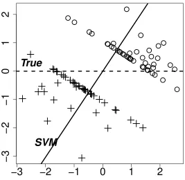
The Support Vector Machine (SVM) is a state-of-the-art powerful classification method proposed by Vapnik (Vapnik, 1995). It has been widely used in bioinformatics and many other disciplines and has achieved a lot of success. Like other classification methods, SVM may suffer from a loss of generalization ability in high dimensional situations as shown by Figure 1 which displays the application of SVM to a high dimensional two class toy
example with class labels +1 and −1. The data have dimension N = 100, with M+ =
45 data vectors from Class +1 represented as circles, and M− = 45 data vectors from
Class −1 represented as plus. The two distributions are nearly standard normal except
that the mean in the first dimension is shifted to +µ and −µ for Class +1 and Class
−1 respectively. Here µ = 1. Figure 1 shows the projections of the data onto the
two-dimensional subspace determined by the first dimension (dashed line) and the normal vector (solid line) of the SVM separating hyperplane. The angle between these two directions can be used to determine the generalization ability of the classifier. A classifier who has good generalization properties should have small angle. For the particular example shown in
c
Figure 1, the angle is 56.6◦. Therefore, projection of a new data vector onto the SVM direction cannot be expected to provide effective discrimination. As mentioned by Marron et al. (2007), the reason is that the estimated SVM classifier is driven only by very particular aspects of the realization of the training data at hand. New data will have their own quite different quirks, which will bear no relation to these.
Hall et al. (2005) studied the High Dimensional Low Sample Size (HDLSS) asymptotics
of SVM and shown that for fixed sample sizeM =M++M−, asN → ∞the angle depends
on the signal size µ which is defined as half of the distance between the means of two
distributions for this example. Assume that µ increases with N as Nγ, then if γ>1/2,
SVM is strongly consistent, i.e., the angle approaches to 0◦; if γ<1/2, SVM is strongly
inconsistent, i.e., the angle approaches to 90◦; ifγ = 1/2, the angle is between 0◦ and 90◦.
Therefore the signal size µhas to be large enough in order to gain some prediction power.
−3
−2
−1
0
1
2
−3
−2
−1
0
1
2
True
SVM
Figure 1: Toy examples, illustrating the performance of SVM on high dimensional data
withN = 100 and sample sizeM =M++M−= 90. The circles denote the data
from Class +1 and and the plus denote the data from Class−1. The dashed line
represents the first dimension which is the true difference in the Gaussian means. The solid line represents the normal vector of SVM separating hyperplane. The
angle between the solid and dashed lines is 56.6◦.
Analogous conclusion has been drawn in the context of unsupervised learning for Princi-pal Component Analysis (PCA). The study of sample covariance matrices is fundamental in multivariate analysis. It is well known that the sample covariance matrix is a consistent
The PCA consistency in HDLSS context (fixed M and N → ∞) was studied in Jung and Marron (2009); Jung et al. (2012) and it was shown that the asymptotic behavior of the Principal Component (PC) directions of sample covariance matrix depend on the size of the
corresponding eigenvalues. Assume that the eigenvalue of the sample covariance matrixλ
increases with N in the order of powerγ, i.e. λ∼Nγ. Then, ifγ>1/2, the corresponding
estimated PC direction is strongly consistent, i.e. the angle between the estimated direction
and its population counterpart is 0◦; if γ<1/2, the corresponding estimated PC direction
is strongly inconsistent, i.e. the angle is 90◦; if γ = 1/2, the angle is random and follows a
certain distribution.
On the other hand, with the development of modern high-throughput technologies, it is
not uncommon to have data where M is comparable in size to N, or substantially larger.
There has been considerable effort to establish asymptotic results for sample eigenvalues
and eigenvectors under the assumption that N and M grow at the same rate, that is,
M/N →α>0 (see review Bai (1999)). The limiting distribution of eigenvalues of the sample covariance matrix was derived in Marcenko and Pastur (1967). Johnstone (2001) studied the distribution of the largest eigenvalue in PCA. Baik and Silverstein (2006) investigated the convergence of the sample eigenvalues and eigenvectors under the spiked population. The degree of discrepancy in terms of the angle between the directions of sample and population eigenvectors was further derived in Paul (2007); Nadler (2008) for both 0<α<1 and α>1 situations. A phenomenon of retarded learning was observed that the angle goes
through a critical phase transition from angle equal to 90◦ for λ<√α to angle less than
90◦ forλ>√α. Therefore, one can only detect signals whose corresponding eigenvalues are
larger than the critical value√αin PCA. More general results have been obtained by Hoyle
and Rattray (2004) and Hoyle and Rattray (2007); Hoyle (2010) for general population covariance matrix.
In the present work, we study the analogous asymptotic results in the joint limitN, M →
∞withM/N =αin the supervised learning context for the SVM classification method. We
focus on the generalization performance of SVM by deriving analytical results for the angle between the estimated direction and the true direction and investigating how this angle
depends on µ,α and other model parameters. We consider a spiked population model and
assume that the data from each class are generated from a purely noise model spiked with a few significant eigenvalues. We derive the analytical results using the replica method developed in statistical mechanics and also compare with numerical simulations on finite size systems. To the best of our knowledge, the present paper is the first that provides not just bounds, but sharp predictions of the asymptotic behavior of the SVM estimators in
the limitN, M → ∞at fixed M/N =α.
An immediate application of our analytical findings is for tuning parameter selection.
SVM is required to solve problem of determining the tuning parameterτ that characterizes
the strength of the penalty term. Cross validation (CV) is a practically useful strategy for handling this task; its basic concept is to evaluate the prediction error by examining the data under control. Smaller values of the CV error are expected to be better to express the generative model of the data. The minimum, if it exists, of the CV error when changing
τ is thus considered to obtain an optimal value of τ. However, conducting CV through
value ofτ base on analytical evaluation for the angle between the estimated SVM direction and true direction which considerably reduces the computational cost. Under the spiked population assumption, smaller angle indicates smaller test error. A surprising finding is that SVM achieves its best performance at small value of the tuning parameter. All analytical results are confirmed by numerical experiments on finite-size systems and our formula is clarified to work well for moderate-size systems.
The rest of this paper is organized as follows: In Section 2, we state SVM in the context of spike population model. The analytical results for large N, M asymptotics are presented. In Section 3, we show the result of numerical experiments to support our analytical results. An application of the proposed tuning parameter selection method to the breast cancer data is also presented in this section. The last section is devoted to the conclusion.
2. Method
In the classification problem, we are given a training dataset consisting of M observations
(xi, yi), for i = 1,· · ·, M. Here xi ∈ RN represents an input vector and yi ∈ {+1,−1}
denotes the corresponding output class label. Each (xi, yi) is an independent random
vec-tor distributed according to a joint distribution function p(x, y). We assume that y has
probability p+ to be +1 and probability p− to be −1 with p++p− = 1. Conditional on
y = +1,−1, x follows multivariate distributions p(x|y = +1), p(x|y = −1) with mean
µ+,µ− and covariance matrices Σ+,Σ−, respectively. Without loss of generality, assume
µ+=−µ− =µ. Similar to linear discriminant analysis, we make an additional simplifying
homoscedasticity assumption Σ+ = Σ− = Σ. Here µ ∈ RN and Σ denotes the N ×N
matrix. Based on this setting, the data from two classes are generated from two multi-variate distributions with the same covariance but different means. The signal size can be
characterized byµ=kµk=
q
PN
j=1µ2j.
We consider a spiked covariance model here. For high dimensional data, typically only few components are biologically important. The remaining structures can be considered as i.i.d. background noise. Therefore, in high-dimensional settings, a collection of data can be modeled by a low-rank signal plus noise structure (Ma, 2013; Liu et al., 2008). We use
a factor analysis model to explain correlations between a set of N variables by means of a
smaller set of K causal factors. Specifically, we assume the following:
Assumption 1 Each observation vector xfrom Class+1can be viewed as an independent instantiation of the following generative model
x=µ+
K
X
m=1
σpλmvmzm+. (1)
Here µ is the mean vector, λm>0, vm ∈RN are orthonormal vectors, i.e. vTmvm = 1 and
vTmvm0 = 0 for m 6= m0, µˆ = µ/µ = v1. The random variables z1,· · ·, zK i.i.d∼ N(0,1).
The vector ={1,· · ·, N} whose elements js are i.i.d random variables withE(j) = 0,
E(2j) =σ2 and E(3j)<∞. The js are independent of zms. The x from Class −1 can be
In model (1), λm represents the strength of the m-th biological component, and σ2
represents the level of background noise. The real biology is typically low-dimensional, i.e. K N. Considering signal as one of the biological components, without loss of generality,
we assume thatµis in the same direction as v1, i.e. ˆµ=v1. Note that the eigenvalueλm
is not necessarily decreasing in m and λ1 is not necessarily the largest eigenvalue. From
(1), the covariance matrix is
Σ=σ2IN + K
X
m=1
σ2λmvmvTm, (2)
whereIN is N-dimensional identity matrix. Although thejs are i.i.d, we didn’t impose any
parametric form for the distribution of j which allows for very flexible covariance
struc-tures for x, and thus the results are quite general. The requirement for the finite third
order moment is to ensure Berry-Esseen central limit theorem applies. The Assumption 1 is also called spiked population model and has been used in many situations, see Baik and Silverstein (2006); Marcenko and Pastur (1967); Johnstone (2001) for examples. Such a population covariance is a finite rank perturbation of multiple of the identity matrix. In other words, all but finitely many eigenvalues of the population covariance matrix are the same. Examples of spiked data include speech recognition (Trevor Hastie, 1995), mathemat-ical finance (LALOUX et al., 2000), wireless communications (Telatar, 1999), and physics of mixture (Sear and Cuesta, 2003).
The task of linear classification is to construct a hyperplanexTw= 0 (w∈RN) so that
the new data vector x is assigned to Class +1 when xTw>0 and Class −1 otherwise. If
the training data are linearly separable, SVM seeks to find this hyperplane such that the minimal distance between the hyperplane and the data point from each class is maximized. The hard-margin SVM solution can be formulated in terms of the following optimization problem
min w
wTw
s.t. yix
T i w
√
N ≥1, i= 1,· · · , M. (3)
To extend SVM to cases in which the data are not linearly separable, we introduce the slack
variables ξi fori= 1,· · ·, M. The soft-margin SVM solution can be formulated in terms of
the following optimization problem
min w
"
wTw+τ
M
X
i=1 ξi
#
s.t. yix
T iw
√
N +ξi ≥1, ξi ≥0, i= 1,· · ·, M, (4)
where the tuning parameterτ determines the trade-off between increasing the margin-size
and ensuring that thexi lie on the correct side of the margin. For sufficiently large values of
τ, the soft-margin SVM will behave identically to the hard-margin SVM. We will show below
that, as τ → ∞, the asymptotic result of soft-margin SVM is the same as the asymptotic
For the setting described in Assumption 1, the normal direction vector of the separating
hyperplane based on Bayes optimal rule is in the same direction as µ. Therefore, the
performance of any classification method can be evaluated by the angle between the normal
direction vector of its separating hyperplane andµ. Propositions 1 and 2 provide the sharp
prediction of the high-dimensional limiting angles for hard-margin SVM and soft-margin SVM respectively.
Proposition 1 Under Assumption 1, in the limitN, M → ∞, with fixedα=M/N, denote θ the angle between µ and w solved from the hard-margin SVM algorithm (3), then cosθ converges to ρ that is determined by the following two nonlinear equations
1−ρ2
1 +λ1ρ2
= α
Z zc
−∞
Dz(zc−z)2, (5)
ρ p
1 +λ1ρ2
= α
Z zc
−∞
Dz(zc−z)
µ σ +
λ1ρ p
1 +λ1ρ2
z !
. (6)
where zc is an unknown parameter needs to be estimated,µ, σ, λ1 are defined in (2), and the standard notation Dz= √dz
2πexp
−z22.
All the proofs are given in the supplementary materials. From equations (5) and (6), we
can solve two unknown parameters ρ and zc given α, µ, σ, andλ1. It is interesting to note
that the results do not depend onλ2,· · ·, λK which means that only the variance along the
signal direction has influence on SVM performance. This observation is also confirmed by extensive simulations in Section 3.1. All the biological components in orthogonal directions have no impact. The nonlinear equations (5) and (6) have no closed form solution. We have to use some numerical algorithms to solve them. As expected, it can be easily checked
from the numerical studies in Section 3 that cos(θ) increases with αas well as the signal to
noise ratioµ/σ, but decreases with λ1.
Proposition 2 Under Assumption 1, in the limitN, M → ∞, with fixedα=M/N, denote θ the angle between µ and w solved from the soft-margin SVM algorithm (4), then cosθ converges to ρ that is determined by the following three nonlinear equations
1−ρ2
1 +λ1ρ2
−αq2ˆτ2
Z zc−qτˆ
−∞
Dz−α
Z zc
zc−qτˆ
Dz(zc−z)2 = 0, (7)
2q−1−αqˆτ
Z zc−qτˆ
−∞
Dzz−α
Z zc
zc−qτˆ
Dz(zc−z)z= 0, (8)
ρF p
1 +λ1ρ2
−αqˆτ µ
σ
Z zc−qˆτ
−∞
Dz−αµ
σ
Z zc
zc−qτˆ
Dz(zc−z) = 0, (9)
where
F = 1−αλ1qτˆ
Z zc−qτˆ
−∞
Dzz−αλ1
Z zc
zc−qˆτ
Dz(zc−z)z,
and
zc=
1/√q0−µρ
σ√1 +λ1ρ
, τˆ= √ στ
q0 √
1 +λ1ρ
Therefore, givenα, λ1, µ, σ, andτ, equations (7), (8), (9) can be used to solve three unknown
parameters ρ, q0, and q. The nonlinear equations (7), (8), and (9) have no closed form
solution. We have to use some numerical algorithms to solve them. Under Assumption 1,
if we further assume thatin (1) follows a normal distribution, then the SVM test error is
ε= Φ
−√ ρ 1+λ1ρ2
µ σ
, where Φ(·) is the cumulative distribution function of N(0,1).
It is interesting to note that, as τ → ∞, the two equations (7) and (9) are equivalent
to (5) and (6) respectively. Therefore, for largeτ, the behavior of soft-margin SVM is the
same as hard-margin SVM. Our simulation studies in Section 3.2 will also confirm this.
For a given dataset, α, λ1, µ, and σ can be estimated, therefore Proposition 2 allows
us to select optimal tuning parameter τ by studying the dependence of ρ on τ for fixed
α, λ1, µ, σ.
We now discuss how to estimateλ1, µ, andσfrom the data. To estimate the background
noise levelσ2, we use a robust variance estimate based on the full matrix of data values (Liu
et al., 2008); that is, for the full set ofM×N entries of the originalM×N data matrixX,
we calculate the robust estimate of scale, the median absolute deviation from the median
(MAD), to estimateσ as
ˆ
σ = MADX
MADN(0,1)
. (10)
Here MADX = median(|xij −median(X)|) and MADN(0,1) = median(|ri −median(r)|),
whereris aM N-dimensional vector whose elements are i.i.d. samples fromN(0,1)
distri-bution.
To estimate λ1, we use the results from Baik and Silverstein (2006) which shows that
in the limit ofM, N → ∞, with fixed α=M/N, the sample eigenvalue ˜λ1 satisfies
˜ λ1
a.s.
−−→
(
(λ1+ 1)
1 +αλ1
1
−1, for λ1> p
1/α,
(1 +p1/α)2−1, for λ1≤
p
1/α. (11)
Therefore, for any finite α, ˜λ1 is not a consistent estimator ofλ1. We use equation (11) to
estimate λ1 as
ˆ λ1 =
1
2 λ˜1− 1
α +
r
˜ λ1−α1
2
−α4
!
, for ˜λ1>1/α+ 2 p
1/α,
p
1/α, for λ˜1 ≤1/α+ 2
p 1/α.
(12)
To estimate µ, let M+, M1 denote the sample sizes of Class +1 and Class−1 respectively.
Defineµc= ¯x+−x¯−, where ¯x+ and ¯x−represent the sample means for Class +1 and Class
−1 respectively. The following Proposition describes the relationship betweenµc and µ.
Proposition 3 Under Assumption 1, in the limit N, M → ∞, with fixed α = M/N, r+ =M+/M, and r−=M−/M, then kµck2 converges to
4µ2+ σ
2 αr+r−
Therefore, we estimateµ as
ˆ µ= 1
2 s
kµˆck2− σˆ2 αr+r−
,
where ˆσ is given from (10) and ˆµc= M1+
PM+
i=1xi−M1−PMi=1−xi is the sample estimation of
µc.
3. Numerical Results
3.1 Hard-margin SVM
2 4 6 8 10
0.2
0.4
0.6
0.8
(a)
µ
cos(
θ
)
0 2 4 6 8 10
0.0
0.2
0.4
0.6
0.8
1.0
(b)
α
cos(
θ
)
0 1 2 3 4 5
0.0
0.2
0.4
0.6
0.8
1.0
(c)
λ1
cos(
θ
)
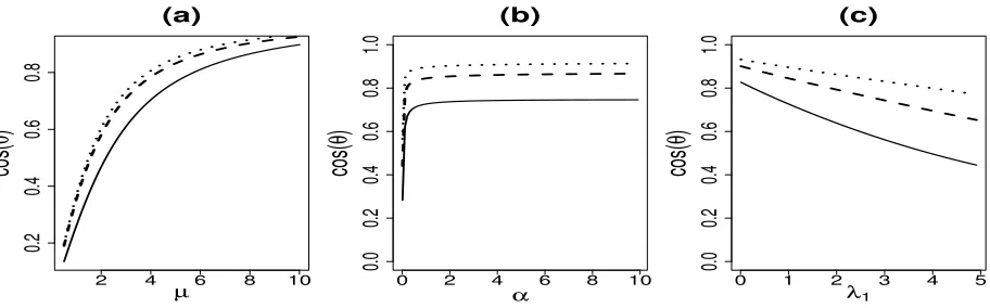
Figure 2: (a) Dependence of cos(θ) on µ for fixed σ = 1, λ1 = 1 and α = 0.1 (solid), 0.5
(dashed), 1.5 (dotted); (b) Dependence of cos(θ) onα for fixedλ1 = 1 andµ= 3
(solid), 5 (dashed), 7 (dotted); (c) Dependence of cos(θ) on λ1 for fixed α = 1
andµ= 3 (solid), 5 (dashed), 7 (dotted).
Figure 2 shows the dependence of cos(θ) on the parameters µ, α, and λ1 based on
numerical solutions of equations (5) and (6). Here θ represents the angle between the
directions of SVM separating hyperplane and Bayes optimal separating hyperplane. For spiked population model (1), the normal vector of Bayes optimal separating hyperplane lies
in the direction ofµ. Discrimination methods whose normal vectorw/kwklies close to this
direction should have good “generalization” properties, i.e., new data will be discriminated
as well as possible. Figure 2(a) shows that, for fixedαandλ1, the classification performance
is improved as we increase the signal size µ. Figure 2(b) shows that, for fixed µ and
λ1, cos(θ) increases with α, indicating that the classification performance is improved by
adding more samples to the training data. For α<1/2, the increasing is faster; for α>2,
when sample size is twice as big as the dimension, adding more samples can not gain too
much power. Figure 2(c) shows that, for fixedµandα, cos(θ) decreases withλ1as expected.
1.5 2.5 3.5 4.5
0.4
0.5
0.6
0.7
0.8
µ
cos(
θ
)
(a)
0.0 1.0 2.0 3.0
0.74
0.76
0.78
0.80
α
cos(
θ
)
(b)
0 1 2 3 4 5
0.3
0.4
0.5
0.6
0.7
λ1
cos(
θ
)
(c)
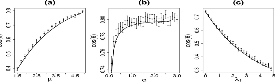
Figure 3: Comparison of analytical calculations with simulation experiments. The solid curves represent the theoretical results, the dots and bars represent the mean
and standard error of the estimated cosθ by applying SVM algorithm (3) to 100
simulated data sets for each parameter setting. In simulations, the dimension
N = 100, the background noise σ = 1. The other parameters are: (a) α =
1, λ1= 2; (b) µ= 5, λ1= 2; (c) α= 1, µ= 2.
To examine the validity of our analysis and to determine the finite-size effect, Figure 3 provides the comparison with numerical simulations on finite size systems. Similar to
Figure 2, we consider the dependence of cos(θ) on three parametersµ,αandλ1 in the plots
in Figure 3 (a), (b), and (c) respectively. Here the dimension of the simulated dataN = 100
and the data are generated according to Assumption 1 withj follows i.i.d standard normal
distribution. We repeat simulation 100 times for each parameter setting. The mean and standard errors over 100 replications are presented. From Figure 3, we can see that our analytical curves show fairly good agreement with the simulation experiment. Thus our analytical formulas (5) and (6) provide reliable estimates even for moderate system sizes. The benefit of these formulas is their computational ease. We also find that the simulation
results for SVM estimators are independent of the choices of orthogonal componentsλm≥2
which further confirms that the analytical results described by Proposition 1 are correct.
3.2 Soft-margin SVM
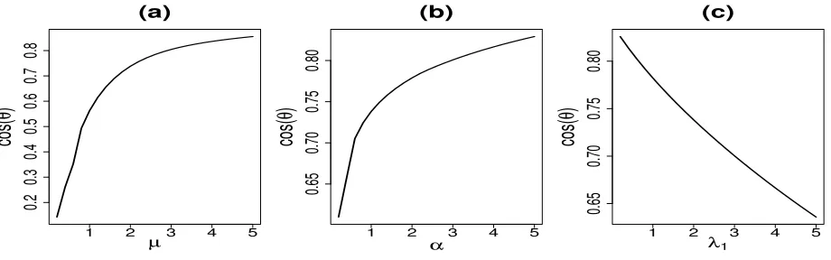
Figure 4 shows the dependence of cos(θ) on the parameters µ, α, and λ1 based on the
solution of nonlinear equations (7), (8), and (9) for fixed τ = 1 and σ = 1. Similar to
Figure 2, the cosθincreases with µand α but decreases withλ1.
To study the the influence of the tuning parameter τ on the performance of the
1 2 3 4 5 0.2 0.3 0.4 0.5 0.6 0.7 0.8 (a) µ
cos(
θ
)
1 2 3 4 5
0.65 0.70 0.75 0.80 (b) α
cos(
θ
)
1 2 3 4 5
0.65 0.70 0.75 0.80 (c) λ1
cos(
θ
)
Figure 4: Dependence of cos(θ) on µ, α, and λ1 forτ = 1 and σ = 1. (a) Dependence of
cos(θ) on µ for fixed λ1 = 2 and α= 1; (b) Dependence of cos(θ) on α for fixed
λ1 = 2 andµ= 2; (c) Dependence of cos(θ) on λ1 for fixedα= 1 and µ= 2.
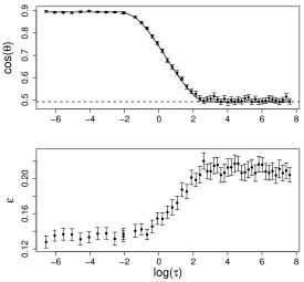
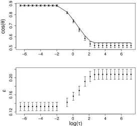
of logτ for fixed α, µ, λ1, and σ. Both the analytical solution based on Proposition 2 and
numerical experiment based on simulated finite dimensional data are provided and they excellently agree with each other. In simulation, we randomly generate a training set and a test set for the given parameter setting, the test error can be obtained by applying the classifier built from the training set to the test set. The results from the summary over 100
replications are given in Figure 5. From the upper panel, it is interesting to note that cosθ
reaches a maximum value as one decreases the tuning parameter τ to a threshold value.
After that value, further decreasingτ cannot change cosθ. On the other hand, if we increase
τ, cosθwill approach the value determined by the hard-margin SVM method as shown by
the dashed line in the upper panel of Figure 5. These observations are further confirmed by
the dependence of test error εon logτ as shown in the lower panel. The test error reaches
a minimum value if we decrease τ to the same threshold value as for cosθ. From equations
(7), (8), and (9), it can be derived that the limiting value of cosθasτ →0 is
ρc= cosθc=
v u u t
α µσ2
1 +α µσ2 (14)
which is independent ofλ1. This finding ofλ1 independence is also confirmed by numerical
simulations with data on finite size systems. Therefore, if in (1) follows a normal
dis-tribution, then the best test error we can achieve using the soft-margin SVM classification
method (4) is Φ
−√ ρc 1+λ1ρ2c
µ σ
.
Koo et al. (2008) studied the asymptotic behavior of the coefficients of the linear SVM
in the limit of M → ∞ withN fixed. They established a Bahadur type representation of
the coefficients and derived their asymptotic normality and statistical variability. Denote
w? the minimizer of the population version of the SVM loss function. It was shown in Koo
−6 −4 −2 0 2 4 6 8
0.5
0.6
0.7
0.8
0.9
cos(
θ
)
−6 −4 −2 0 2 4 6 8
0.12
0.16
0.20
log(τ)
ε
Figure 5: Upper panel: compare theoretical result with simulation experiment for the
de-pendence of cos(θ) on tuning parameter log(τ) for fixed α = 1, µ = 2, σ = 2,
and λ1 = 2. The solid line is the theoretical curve, the dots and bars represent
the mean and standard error based on 100 simulated data sets at each parameter
setting. In simulation, the dimension N = 100. The dashed line represents the
value based on the hard-margin SVM solution from equations (5) and (6). Lower
under the spiked population setting (1). Therefore ρ → 1 as M → ∞ with N fixed. This
can be confirmed in (14) by letting α → ∞ on the right hand side. On the other hand,
if we let N → ∞ with M fixed, from (14) we get ρc → 0 if µ/
√
N → 0 and ρc → 1 if
µ/√N → ∞. This confirms the results of Hall et al. (2005) for HDLSS setting. Therefore,
our asymptotic results are more general with both traditional and HDLSS asymptotics as special cases.
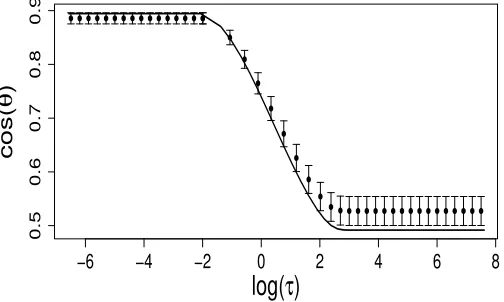
The analytical results in Figure 5 are based on the true values forα, λ1, µand σ which
ultimately need to be estimated from the given data. In Figure 6 we provide the comparison between the results using the true values and the results using the estimated values for µ, α, λ1 andσ. For each simulated data, we first estimateµ, α, λ1 and σand then use them to derive theoretical results. Figure 6 indicates that the influence of moderate estimation errors in the parameters is small.
−6 −4 −2 0 2 4 6 8
0.5
0.6
0.7
0.8
0.9
log(
τ
)
cos(
θ
)
Figure 6: Comparison between the results using the true values and the results using the
estimated values for parameters. Here the true parameter values areα= 1,µ= 2,
σ= 1, and λ1 = 2. The solid curve represents the results derived using the true
values. The dots and bars represent the means and standard errors of the cosθ
values derived using the estimated parameters for 100 simulated data sets.
Although Figure 5 suggests that, for spiked population model, the best performance of
SVM is achieved at the smallest valueτ, in practice, using too tinyτ could cause difficulties
in numerically solving the optimization problem. In order to provide a practical
recommen-dation for the tuning parameter, we need to estimate the threshold value τc at which the
limiting value cosθc is almost achieved, i.e. the elbow point in Figure 5. More precisely,
τc is defined as τc = max{τ : ρ(τ) = ρc}. In practice, we can compute τc by numerically
finding the largestτ that can give cosθ=ρcand use it as a guideline for choosingτ. Figure
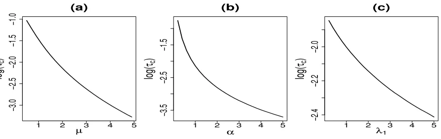
7 displays the change of logτcas functions of the parametersµ, α, λ1. It is shown that logτc
decreases with all three parameters.
3.3 Check the model assumptions
1 2 3 4 5
−3.0
−2.5
−2.0
−1.5
−1.0
(a)
µ
log(
τ
c)
1 2 3 4 5
−3.5
−2.5
−1.5
(b)
α
log(
τ
c)
1 2 3 4 5
−2.4
−2.2
−2.0
(c)
λ1
log(
τ
c)
Figure 7: (a) Dependence of log(τc) on µ for fixed λ1 = 2 and α = 1; (b) Dependence of
log(τc) onα for fixedλ1 = 2 andµ= 2; (c) Dependence of log(τc) onλ1 for fixed
α= 1 andµ= 2.
study the validity of our method in situations where these assumptions are not true. Figure 8 is for situation where the two covariance matrices from the positive and negative classes
are different. In simulation, we first generateM samples fromN(0, σ2I
p) distribution. Then
M/2 of them are shifted by µin x1 direction to form the positive class and the remaining M/2 are shifted by −µ inx1 direction to form the negative class. Both classes are further
divided into two subclasses with sample size M/4 for each. In the positive class, the two
subclasses are separated by shifting in x2 direction by µ and −µ respectively. Similarly,
the two subclasses in the negative class are separated by shifting in x3 direction by µ
and −µ respectively. The data generated in this way satisfies the spiked assumption but
the two classes have different covariances. Figure 8 shows that the theoretical estimation and direct computation agree fairly well with each other. We have tried several different
settings for µ, α and σ and got similar results. Therefore, our method is fairly robust to
homoscedasticity as long as the spiked condition (1) holds for the covariance matrices of both classes.
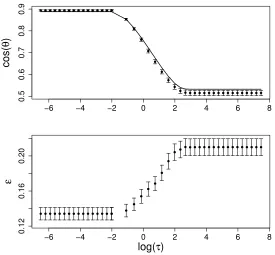
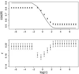
Figures 9, 10, and 11 are for situations where the spiked assumption is violated. In
simulation, we first generateM samples fromN(0,Σ) distribution. ThenM/2 of them are
shifted by µ in x1 direction to form the positive class and the remaining M/2 are shifted
by−µinx1 direction to form the negative class. The covariance matrixΣis diagonal with
the ith eigenvalue equal to iσ2 fori ≤K and σ2 for i>K. The spiked condition requires K p. If we increase K, the spiked condition can be violated. Figures 9, 10, and 11
show the results for K = 0.1N, K = 0.3N, and K = 0.5N respectively. For situations
where the number of uncommon eigenvalues K is less than 10% of the total number of
variables N, our method can provide quite accurate estimation for cosθ and also bigger
cosθ corresponds to smaller test error as illustrated in Figure 9. For situations where K
is 30% ofN, our method can still provide reasonable estimation for cosθ, but cosθ cannot
−6 −4 −2 0 2 4 6 8
0.5
0.6
0.7
0.8
0.9
cos(
θ
)
−6 −4 −2 0 2 4 6 8
0.12
0.16
0.20
log(τ)
ε
Figure 8: Comparison of theoretical prediction with direct computation for simulated data
using parametersα= 1, µ= 2, σ= 2, and λ1 = 2. In simulation, the covariances
smaller test error as illustrated in Figure 10. For situations where K is 50% of N, our
method cannot provide estimation for cosθ. Moreover, cosθand εbehavior in an opposite
way, i.e. smaller cosθcorresponds to smaller test error as illustrated in Figure 11.
−6 −4 −2 0 2 4 6
0.5
0.6
0.7
0.8
0.9
cos(
θ
)
−6 −4 −2 0 2 4 6
0.12
0.16
0.20
log(τ)
ε
Figure 9: Comparison of theoretical prediction with direct computation for simulated data
using parameters α= 1, µ= 2, σ= 2, and λ1 = 2. In simulation, the number of
the uncommon eigenvaluesK is equal to 10% of the total number of variables N.
In summary, our simulations indicate that the proposed method depends on the spiked assumption but is not sensitive to the homoscedasticity violation. The spiked assumption is based on factor analysis which is one of the most useful tools for modeling common dependence among all the variables. In genetics, factor analysis modeling appeared to be useful tools to investigate the dependence structure in high-dimensional microarray data. It can fit the data with covariance matrix governed by linkage disequilibrium patterns (Rochat et al., 2007). For data set which cannot be modeled using spiked population, our results indicate that further exploring the data structure is useful for understanding the classification performance.
3.4 Real Data
−6 −4 −2 0 2 4 6
0.5
0.6
0.7
0.8
0.9
cos(
θ
)
−6 −4 −2 0 2 4 6
0.14
0.18
0.22
log(τ)
ε
Figure 10: Comparison of theoretical prediction with direct computation for simulated data
using parametersα= 1, µ= 2, σ= 2, andλ1 = 2. In simulation, the number of
the uncommon eigenvalues K is equal to 30% of the total number of variables
−5 0 5
0.3
0.5
0.7
0.9
cos(
θ
)
−5 0 5
0.25
0.35
log(τ)
ε
Figure 11: Comparison of theoretical prediction with direct computation for simulated data
using parametersα= 1, µ= 2, σ= 2, andλ1 = 2. In simulation, the number of
the uncommon eigenvalues K is equal to 50% of the total number of variables
−10 −5 0 5
0.4
0.6
0.8
cos(
θ
)
−10 −5 0 5
0.22
0.26
0.30
log(τ)
ε
Figure 12: Upper panel: theoretical prediction of the dependence of cos(θ) on tuning
pa-rameter log(τ) based on the solutions from equations (7), (8) and (9) using
parameters estimated from the breast cancer data. Lower panel: dependence of
cross-validation errorεon tuning parameter log(τ). The dots and bars represent
We consider LumA as Class +1 and LumB as Class -1. Assume the data are generated based on model (1), using the method discussed in Section 2, we obtain the following
parameter estimations: ˆµ = 3.80, ˆσ = 2.32, ˆλ1 = 4.06, α = 4.20, N = 56, M = 235,
M+ = 154, M− = 81. The upper panel of Figure 12 shows the analytical curve for the
dependence of cosθonτ. It shows that if we chooseτ less than 6.19×10⁻³, we can get the
smallest angle. The lower panel of Figure 12 shows the dependence of the cross validation
errors as a function of τ. The cross validation errors are computed by randomly splitting
the data into two parts, 90% for training and 10% for test. The mean and standard error over 100 random splitting are reported in the lower panel of Figure 12. It shows that the
cross validation error can achieve minimum value if τ is less than around 5×10⁻³. The
two results are consistent with each other and similar to the previous simulation results as shown in Figure 5. This indicates that model (1) is a reasonable assumption for this data set.
4. Conclusion
In this study, we examine the asymptotic behavior of SVM in the limit of N, M → ∞
with fixed α = M/N. We investigate the estimators of both the hard-margin SVM and
the soft-margin SVM methods. Our focus is on the angle between the direction of the esti-mated separating hyperplane and the Bayes optimal separating hyperplane. Under spiked population model assumption, we analytically evaluate the relation between this angle and the SVM tuning parameter. On the basis of this finding, a new method of selecting tuning parameter is developed for analyzing high dimensional data which significantly reduces the computational cost. The analytical calculations are compared with numerical simulations on finite-size systems and the agreement between the numerical data and the analytical result is fairly good, and thus, our formulas are validated. Although the asymptotic results that we have obtained apply only to the spiked population model, they have shed a new light on the asymptotic behavior of SVM and can also improve the practical use of SVM in various aspects. For situations where the spiked model cannot be applied, one possible solution is to use the generalized spiked population model proposed in Bai and Yao (2012) to re-derive our results. This is one of our future research topics.
Acknowledgments
The author would like to thank the Action Editor Professor Xiaotong Shen and three review-ers for their constructive comments and suggestions, which led to substantial improvements of the presentation of this paper.
References
Z. D. Bai. Methodologies in spectral analysis of large-dimensional random matrices, a
review. Statistica Sinica, 9:611–677, 1999.
Zhidong Bai and Jianfeng Yao. On sample eigenvalues in a generalized spiked population
model. Journal of Multivariate Analysis, 106:167 – 177, 2012.
Jinho Baik and Jack W. Silverstein. Eigenvalues of large sample covariance matrices of
spiked population models. Journal of Multivariate Analysis, 97(6):1382 – 1408, 2006.
Peter Hall, J. Marron, and Amnon Neeman. Geometric representation of high
dimen-sion, low sample size data. Journal of the Royal Statistical Society: Series B (Statistical
Methodology), 67(3):427–444, 2005.
D. C. Hoyle and M. Rattray. Principal-component-analysis eigenvalue spectra from data
with symmetry-breaking structure. Phys. Rev. E, 69:026124, 2004.
D. C. Hoyle and M. Rattray. Statistical mechanics of learning multiple orthogonal signals:
Asymptotic theory and fluctuation effects. Phys. Rev. E, 75:016101, 2007.
David C Hoyle. Statistical mechanics of learning orthogonal signals for general covariance
models. Journal of Statistical Mechanics: Theory and Experiment, 2010(04):P04009,
2010.
Iain M. Johnstone. On the Distribution of the Largest Eigenvalue in Principal Components
Analysis. The Annals of Statistics, 29(2):295–327, 2001.
S. K. Jung and J. S. Marron. PCA consistency in high dimension, low sample size context. The Annals of Statistics, 37:4104–4130, 2009.
Sungkyu Jung, Arusharka Sen, and J.S. Marron. Boundary behavior in high dimension, low
sample size asymptotics of PCA. Journal of Multivariate Analysis, 109:190 – 203, 2012.
Ja-Yong Koo, Yoonkyung Lee, Yuwon Kim, and Changyi Park. A bahadur representation of
the linear support vector machine. Journal of Machine Learning Research, 9:1343–1368,
June 2008.
LAURENT LALOUX, PIERRE CIZEAU, MARC POTTERS, and JEAN-PHILIPPE
BOUCHAUD. Random matrix theory and financial correlations. International
Yufeng Liu, David Neil Hayes, Andrew Nobel, and J. S Marron. Statistical significance of
clustering for high-dimension, low-sample size data. Journal of the American Statistical
Association, 103(483):1281–1293, 2008.
Yufeng Liu, Hao Helen Zhang, and Yichao Wu. Hard or soft classification? large-margin
unified machines. Journal of the American Statistical Association, 106(493):166–177,
2011.
Zongming Ma. Sparse principal component analysis and iterative thresholding. Ann.
Statist., 41(2):772–801, 04 2013.
V. A. Marcenko and L. A. Pastur. Distribution of eigenvalues for some sets of random
matrices. Mathematics of the USSR-Sbornik, 1(4):457–483, April 1967.
J. S. Marron, M. Todd, and J. Ahn. Distance-weighted discrimination. Journal of the
American Statistical Association, 102:1267–1271, 2007.
Boaz Nadler. Finite sample approximation results for principal component analysis: A
matrix perturbation approach. The Annals of Statistics, 36(6):2791–2817, 2008.
The Cancer Genome Atlas Research Network. Comprehensive genomic characterization
defines human glioblastoma genes and core pathways. Nature, 455:1061–1068, 2008.
Debashis Paul. Asymptotics of sample eigenstructure for a large dimensional spiked
covari-ance model. Statistica Sinica, 17:1617–1642, 2007.
Xingye Qiao and Lingsong Zhang. Flexible high-dimensional classification machines and
their asymptotic properties. Journal of Machine Learning Research, 16:1547–1572, 2015.
R. H. Rochat, L. de las Fuentes, G. Stormo, V. G. Davila-Roman, and C. Charles Gu. A novel method combining linkage disequilibrium information and imputed functional
knowledge for tagsnp selection. Hum Hered, 64(4):243–249, 2007.
Richard P. Sear and Jos´e A. Cuesta. Instabilities in complex mixtures with a large number
of components. Phys. Rev. Lett., 91:245701, Dec 2003.
E. Telatar. Capacity of multi-antenna Gaussian channels. Eur. Trans. Telecomm. ETT, 10
(6):585–596, November 1999.
Robert Tibshirani Trevor Hastie, Andreas Buja. Penalized discriminant analysis. The
Annals of Statistics, 23(1):73–102, 1995.