Image Restoration using Hybrid Neuro- Fuzzy Filter

Image Restoration using Hybrid

Neuro-Fuzzy Filter

Dr C.Sugapriya

Assistant Professor, Queen Mary’s College, Chennai.

ABSTRACT

Digital images are often corrupted by impulse noise during image acquisition and/or transmission due to a number of non idealities encountered in image sensors and communication channels. In most image processing applications, it is of vital importance to remove the noise from the image data because the subsequent image processing tasks (such as segmentation and feature extraction, object recognition, etc.) are severely degraded by noise. A new operator for restoring digital images corrupted by impulse noise is presented. The proposed operator is a simple recursive switching median filter guided by neuro-fuzzy network functioning as an impulse detector. The proposed operator is a hybrid filter obtained by appropriately combining a median filter, an edge detector, and a neuro-fuzzy network. The internal parameters of the neuro-fuzzy network are adaptively optimized by training. The most distinctive feature of the proposed operator over most other operators is that it offers excellent line, edge, detail, and texture preservation performance while, at the same time, effectively removing noise from the input image. Extensive simulation experiments show that the proposed operator may be used for efficient restoration of digital images corrupted by impulse noise without distorting the useful information in the image.

Keywords: Peak Signal to Noise Ratio, Image Quality, Mean Square Error, Fuzzy Logic

1. INTRODUCTION

1.1 NEURAL NETWORKS

Neural networks, with their remarkable ability to derive meaning from complicated or imprecise data, are used to extract patterns and detect trends that are too complex to be noticed by either humans or other computer techniques. A trained neural network is thought of as an “expert” in the category of information it is given to analyze. This expert provides projections given new situations of interest.

An artificial neural network (ANN) is an information-processing paradigm that is inspired by the way biological nervous system, such as the brain, process information. The key element of this paradigm is the novel structure of the information processing system it is composed of a large number of highly inter connected processing elements (neurons) working in unison to solve specific problems.

An artificial neuron is a device with many inputs and one output. The neuron has two modes of operation; the training mode and the using mode. In the training mode, the neuron is trained to fire (or not), for particular input patterns. In the using mode, if a taught input pattern is detected at the input, its associated output becomes the current output. If the input pattern does not belong in the taught list of input patterns, the firing rule is used to determine whether to fire or not.

All learning methods used for adaptive neural networks are classified into two major categories:

Supervised learning

It incorporates an external teacher, so that each output unit conforms to its desired response to input signals. During the learning process information is required. Paradigms of supervised learning include error correction learning, reinforcement learning and stochastic learning. An important issue connecting supervised learning is the problem of error convergence, i.e. the minimization of error between the desired and computed unit values. The aim is to determine the set of weights that minimizes the error. One well known method, which is common to many learning paradigms, is the least mean square (LMS) convergence.

Unsupervised learning:

It uses no external teacher and is based upon only local information. It is also referred to as organization, in the sense that it self-organizes data presented to the network and detects their emergent collective properties.

1.1.1 BACK PROPAGATED DELTA RULE NETWORKS (BP)

It is a development from the simple delta rule in which extra hidden layers (layers additional to the input and output layers, not connected externally) are added. The network topology is feed forward: i.e. loop-free. Connections are allowed from the input layer to the first hidden layer; from the first hidden layer to the second, and so on, up to the last hidden layer at least to the output layer. In the typical back propagation networks, the hidden layer learns to recode (or to provide a representation for) the inputs. More than one hidden layer is used.

1.1.2 RADIAL BASIS FUNCTION NETWORKS (RBF)

Radial basis function networks learn arbitrary mapping; the primary difference is in the hidden layer.

RBF hidden layer units have a receptive field that has a center; that is, a particular input value at which they have a maximal output. The output tails off as the input moves away from this point. The hidden unit function is a Gaussian function. Networks are also feed forward, but have only one hidden layer.

2. FUZZY LOGIC

Fuzzy Logic provides a simple way to arrive at a definite conclusion based upon vague, ambiguous, imprecise, noisy or missing information. It incorporates a simple, rule based IF X AND Y THEN Z approach to solve a problem. The fuzzy logic is empirically based, relying on operator‟s experience and not on their technical understanding of the system. The skilled operator‟s heuristic knowledge in the fuzzy logic system is realized with appropriate membership functions.

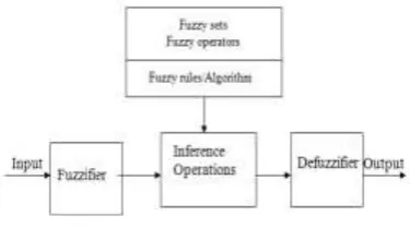
Fig.2 General Fuzzy System

The fuzzy is composed of a knowledge based that contains fuzzy rules, the definition of the fuzzy membership functions, the type of fuzzy operators being used and an inference engine which evaluates the fuzzy rules. But in addition, it also has a fuzzifier, which represents a real-valued input signal as a fuzzy set, and a

defuzzifier that compresses the information contained in a fuzzy output distribution to a single value.

The membership function takes values between 0 and 1 and is a graphical representation of the magnitude of participation of each input. It associates a weighting with each of the inputs that are processed, define functional overlap between inputs, and ultimately determines an output response. The rules use the input membership values as weighting factors to determine their influence on the fuzzy output sets of the final output.

2.1 MEMBERSHIP FUNCTION:

The membership function values need not always be described by discrete values. Quite often, these turn out to be as described by a continuous function. The membership function can be given mathematically as,

μĂ (x) = 1 / (1+x)2 . . ( 1)

Different shapes of membership functions exist. Here we use bell shaped membership function

3. HYBRID NEURO FUZZY FILTER:

Fig .3 Hybrid Filter

3.1 HYBRID MEDIAN FILTER:

The median filter is a simple rank selection filter that outputs the median of the pixels contained in its filtering window. I have made literature survey some of they are Fumitaka et al. (2015) demonstrated the zero-mean white Gaussian noise removal method using high-resolution frequency analysis. It is hard to separate an original image component from a noise component at what time using discrete Fourier transform (DFT) or discrete cosine transform (DCT) for analysis. Two-dimensional non-harmonic analysis (2D NHA) is a high-resolution frequency analysis technique that improves noise removal accuracy because of its sidelobe reduction feature.

external patch priors may yield a better patch prior. In this particular, it first learn the generic Gaussian mixture model from a collection of training images and then adapt the model to the given image by simultaneously adding additional components and refining the component parameters.

Ruiqin Xiong et al. (2016) discussed the new image denoising algorithm based on adaptive signal modeling and regularization and also it improves the quality of images by regularizing each picture patch using band wise distribution modeling in transform domain. The simulated experimental results show that the presented scheme outperforms several state-of-the-art denoising methods in both the objective and the perceptual qualities.

Jian Ji & Yang Li (2016) presented the Synthetic aperture radar (SAR) image denoising. The basis of SAR image can be estimated by Independent component analysis and these bases can be divided into two different subspaces (noise and real signal subspaces) through a linear classifier. According to various results measured by Bootstrap, corresponding Maximum a posterior probability (MAP) filter will be selected for image denoising, using the noise model‟s parameter for adaptive filtering technique. The simulated experiments show that the image processed by this presented method can achieve a better visual perception and objective evaluation results.

The hybrid median filter does not excessively smooth image details and typically provides the superior visual quality of the filtered image. It has multiple step brightness algorithm. The input-output relationship of the median filter may be defined as follows:

Let x[r,c] denote the luminance value of the pixel at location (r,c) of the noisy input image.

Table 1 3×3 Pixel Filtering Window (N = 1)

X[r-1,c-1] X[r-1,c] X[r-1,c+1]

X[ r ,c-1] X[ r , c] X[ r , c+1]

X[r+1,c-1] X[r+1,c] X[r+1,c+1]

Here, r and c are the row and the column indices, respectively, with 1 ≤ r ≤ R and 1 ≤ c≤ C for an input image having a size of R-by-C pixels. Let WN[r,c] represent the group of

pixels contained in a filtering window centered at

location (r,c) of the noisy input image and having the size of (2N+1)-by-(2N+1) pixels.

WN[r,c] = {x[ r+p, c+q ]│( p, q ) = -N, .N} . . .

. .(2)

Where N is a positive integer number related with the size of the filtering window and p and q are integer indices each individually ranging from –N to N.

The output of the median filter is equal to the median of the pixels contained in the filtering window WN[r,c]

m[r,c] = Median (WN[r,c]).. . (3)

3.2 CANNY EDGE DETECTOR

There are a number of different edge detectors in use. In previous chapter, however, a major drawback of almost all of these edge detectors is that their detection performance is significantly degraded by noise, which makes them inappropriate for use in the structure of the proposed hybrid filter.

Recently, a novel edge detector for use with noisy images is introduced. It has been shown that this detector is capable of extracting edges from digital images corrupted by impulse noise without requiring a prefiltering of the input image. Therefore, this edge detector is employed as the edge detector in this work.

The edge detector comprises four identical subdetectors. Each subdetector is a Sugeno type fuzzy system similar to the one used in the structure of the noise removal operator proposed in this project. The four subdetectors individually process four different pixel neighborhoods in horizontal, vertical, left diagonal and right diagonal directions, respectively. The input data to the subdetectors are, therefore, the pixel luminance values within a particular neighborhood. The outputs if the subdetectors are fed to a postprocessor, which generates the final edge image. The postprocessor decides whether the center pixel of a given 3×3 analysis window is an edge pixel or not. The postprocessor actually calculates the average value of the four subdetector outputs and compares this value with a threshold to decide whether the pixel is an edge pixel.

A. CANNY ALGORITHM

The canny detector is the most powerful edge detector provide by function edge. This algorithm can be summarized as follows: 1. The image is smoothed using a Gaussian

filter with a specified standard deviation, σ, to reduce noise.

2. The local gradient, g ( x, y) = [Gx2 + Gy2]1/2,

3. α ( x, y) = tan-1(Gy/Gx), are computed at

each point. Any of the techniques can be used to compute Gx and Gy. An edge point

is defined to be a point chose strength is locally maximum in the direction of the gradient.

4. The edge points determined in (2) give rise to ridges in the gradient magnitude image. The algorithm then tracks along the top these ridges and sets to zero all pixels that are not actually on the ridge top so as to give a thin line in the output, a process known as nonmaximal suppression. The ridge pixels are then thresholded using two thresholds, T1 and T2, with T1 < T2. Ridge pixels with values greater than T2 are said to be “strong” edge pixels. Ridge pixels with values between T1 and T2 are said to be “weak” edge pixels.

The syntax for the Canny edge detector is [ g , t ] = edge (f, „canny‟, T, sigma) where T is a vector, T = [T1, T2], containing the thresholds explained in step 3 of the preceding procedure, and sigma is the standard deviation of the smoothing filter. If t is included in the output argument, it is a two-element vector containing the two threshold values used by the algorithm. The rest of the syntax is similar to the other methods, including the automatic computation of the thresholds if T is not supplied. The default value for the sigma is 1.

3.3 NEURO-FUZZY SYSTEM:

In the last few years, there has been growing research interest in the applications of soft computing techniques, such as neural networks and fuzzy systems, to the problems in digital image processing. Indeed neuro-fuzzy (NF) systems offer the ability of neural networks to learn from examples and the capability of fuzzy systems to model the uncertainty which is inevitably encountered in noisy environments. Therefore NF systems may be utilized as very powerful tools for the detection and/or removal of impulse noise from digital images, provided that appropriate network structure and processing strategies are employed. Hence, a number of nonlinear impulse noise removal operators based on soft computing techniques have also been proposed. One important class of these operators is fuzzy filters based on fuzzy then and if-then-else rules.

These operators usually employ a set of fuzzy rules for the detection of the impulse noise in a given filtering window, and an appropriate mechanism for its removal. Although they offer better noise removal performance than the median-based operators, they are inherently heuristic the determination of fuzzy rules may be quite complicated especially when the noise

density is high. In order to overcome this difficulty, methods that allow the determination of internal parameters of the fuzzy filter by training have also been presented. However the structures of these systems are much more complex and the required filtering window size is usually larger than other methods. In addition, multi-output network topologies and the use of two-dimensional membership functions even more increase the complexity of these systems.

A. NEURO FUZZY NETWORK:

The NF network used in the structure of the proposed hybrid filter acts like a fusion operator and attempts to construct an enhanced output image by combining the information from the median filter, the edge detector and the noisy input image. The rules of fusion are represented by the rules in the rule base of the NF network and the fusion process is implemented by the fuzzy inference mechanism of the NF network.

The NF network is the first order Sugeno type fuzzy system with three inputs and one output. Sugeno-type fuzzy systems are popular general nonlinear modeling tools because they are very suitable for tuning by optimization and they employ polynomial type output membership functions, which greatly simplifies defuzzification process.

The input-output relationship of the NF network is as follows. Let X1, X2, X3 denote

the inputs of the NF network and Y denote its output. The fuzzy inference is performed on the noisy input image pixel by pixel. Each noisy pixel is independently processed by the median filter and the edge detector before being applied to the NF network. Hence, in the structure of the proposed operator, X1 represents the output of

the median filter for the noise input pixel, X2

represents the output of the edge detector for the noise input pixel, X3 represents the noisy pixel

itself. Each possible combination of inputs and their associated membership functions is represented by a rule in the rule base of the NF network. Since the NF network has three inputs and each input has three membership functions, the rule base contains a total of 27 (33) rules, which are as follows.

1. If (X1 is M11) and (X2 is M21) and (X3 is

M31) then

R1 = F1(X1, X2, X3).

2. If (X1 is M11) and (X2 is M21) and (X3 is

M32) then

R2 = F2 (X1, X2, X3).

3. If (X1 is M11) and (X2 is M21) and (X3 is

M33) then

4. If (X1 is M11) and (X2 is M22) and (X3 is

M31) then

R4 = F4 (X1, X2, X3).

5. If (X1 is M11) and (X2 is M22) and (X3 is

M32) then

R5 = F5 (X1, X2, X3).

. . .

27. If (X1 is M13) and (X2 is M23) and (X3 is

M33) then R27 = F27 (X1, X2, X3)

where Mij denotes the j th membership function

of the i th input, Rk denotes the output of the k th

rule, and Fk denotes the k th output membership

function, with i = 1, 2, 3; j = 1, 2, 3; and k = 1, 2, 3, ….., 27. The input member ship functions are general bell type

…..(4) The output membership functions are linear Fk (u1, u2, u3 ) = dk1u1 + dk2u2 + dk3u3 + dk4

. . . (5)

Where u, u1, u2, & u3 are format parameters, & the parameters, a, b, c, & d are constants that characterize the shape of the membership functions. The optimal values of these parameters are determined by training.

It should be noted that there is no analytical method to determine the optimal number of the membership functions. The optimal number of the membership functions is usually determined heuristically and verified experimentally. A smaller number yields lower complexity and shorter training time, but poor performance. On the other hand, a greater number yields better performance, but higher complexity and much longer training time. It has been experimentally determined that three membership functions offer a very good cost / benefit balance.

The output of the NF network is the weighted average of the individual rule outputs. The weighting factor wk of each rule is

calculated by evaluating the membership expressions in the antecedent of the rule. This is accomplished by first converting the input values to fuzzy membership values by utilizing the input membership functions and then applying the and operator to these membership values. The and operator corresponds to the multiplication of input membership values.

Hence, the weighting factors of the rules are calculated as follows

w1 = M11(X1). M21(X2). M31(X3)

w2 = M11(X1). M21(X2). M32(X3)

w3 = M11(X1). M21(X2). M33(X3)

w4 = M11(X1). M22(X2). M31(X3)

w5 = M11(X1). M22(X2). M32(X3)

. .

w27 = M13(X1). M23(X2). M33(X3)

Original Training Image

Fig.4 Training of Neuro-Fuzzy Network

Original Noisy (corrupted by 30% Impulse noise)

Fig.5 Training images

Once the weighting factors are obtained, the output of NF network can be found by calculating the weighted average of the individual rule outputs

……..(5)

B. TRAINING OF THE NEURO-FUZZY NETWORK:

output of the ideal noise filter which, by definition, completely removes the noise from its input image. The ideal noise filter is conceptual only and does not necessarily exist in reality. It is only the output of the ideal noise filter that is necessary for training, and this is represented by the original (noise-free) training image.

Fig.4 shows the images used for training. Only one image (image pair) is used in training. The image shown in Fig.5 (a) is the original training image, which is a 128×128 pixel artificial image that can easily be generated in a computer. Each square box in this image has a size of 4×4 pixels and the 16 pixels contained within each box have the same luminance value, which is a random integer number uniformly distributed

in [0,255]. The image in Fig.5 (b) is the noisy training image by impulse noise of 30% noise density.

Although the density of the corrupting noise is not very critical regarding training performance, it is experimentally observed that the proposed operator exhibits the best filtering performance when the noise density of the noisy traning image is equal to the noise density of the actual noisy input image to be restored. It is also observed that the performance of the proposed operator gradually decreases as the difference between the two noise densities increases. Hence, in order to obtain a stable filtering performance for a wide range of filtering noise densities, very low and very high values for traning noise density should be avoided since it is usually impossible to know the actual noise density of a corrupted image in a real practical application.

Results of extensive simulation experiments indicate that very good filtering performance is easily obtained for all kinds of images corrupted by impulse noise with a wide range of noise densities provided that the noisy training image has a noise density around 30%.

The images in Fig.5 (a) and (b) are employed as the input and the target (desired) images during training, respectively. The parameters of the NF network are then iteratively tuned by using the Levenberg-Marquardt optimization algorithm so as to minimize the learning error.

Once the training of the NF network is completed, its internal parameters are fixed and the network is combined with the median filter and the edge detector to construct the proposed hybrid filter Fig.4

3.4 FILTERING OF THE NOISY IMAGE:

The noisy input image is processed by sliding the 3×3 filtering window on the image. This filtering window is also the filtering window for both the median filter and the edge detector. The window is started from the upper-left corner of the noisy input image, and moved rightwards and progressively downwards in a raster scanning fashion. For each filtering window, the nine pixels contained within the window are first fed to the median filter and the edge detector in the structure. Next, the center pixel of the filtering window and the outputs of the median filter and the edge detector are applied to the appropriate inputs of the NF network. Finally, the restored luminance value for the center pixel of the filtering window is obtained at the output of the NF network by using the fuzzy inference mechanism. The simulation result of proposed as illustrated in Fig 6.

Fig.6 Simulation result of Proposed Method

4. CONCLUSION

structure of the proposed operator yields slightly better performance, but also increases the computational load.

Based on these observations, it is concluded that the proposed operator can be used as a powerful tool for efficient removal of impulse noise from digital images without distorting the useful information within the image.

REFERENCES:

1. M. Emin Yuksel, „A Hybrid Neuro-Fuzzy Filter for Edge Preserving Restoration of Images Corrupted by Impulse Noise‟, IEEE Transactions On Image Processing, Vol. 15, No. 4, April 2006.

2. Rafael C. Gonzalez, Richard E. Woods, Steven L. Eddins (2005)„Digital Image Processing using MATLAB‟, Pearson Education (Singapore) Pvt.Ltd., Third Edition.

3. Rafael C. Gonzalez, Richard E. Woods (2001) „Digital Image Processing‟, Pearson Education (Asia) Pvt.Ltd, Seventh Indian Reprint.

4. Stamatios V. Kartalopoulos (2000) „Understanding Neural Networks and Fuzzy Logic‟, Prentice Hall of India (New Delhi) Pvt. Ltd.

5. Fumitaka Hosotani, Yuya Inuzuka, Masaya

Hasegawa, Shigeki Hirobayashi & Tadanobu Misawa 2015, „Image Denoising With Edge-Preserving and Segmentation Based on Mask NHA‟, IEEE Transactions on Image Processing, vol. 24, no. 12, pp. 6025-6033.

6. Jian Ji & Yang Li 2016, „An Improved

SAR Image Denoising Method Based on Bootstrap Statistical Estimation with ICA Basis‟, Chinese Journal of Electronics, vol. 25, no. 4, pp. 786-792. 7. Ruiqin Xiong, Hangfan Liu, Xinfeng Zhang, Jian

Zhang, Siwei Ma, Feng Wu & Wen Gao 2016, „Image Denoising via Bandwise Adaptive Modeling and Regularization Exploiting Nonlocal Similarity‟, IEEE Transactions on Image Processing, vol. 25, no. 12, pp. 5793-5805.