Two-Stage Label Embedding via Neural Factorization Machine for Multi-Label Classification

(1)

The Thirty-Third AAAI Conference on Artificial Intelligence (AAAI-19)

Two-Stage Label Embedding via Neural

Factorization Machine for Multi-Label Classification

Chen Chen,

1,3∗

Haobo Wang,

1,3*

_{Weiwei Liu,}

4

_{Xingyuan Zhao,}

1,3

_{Tianlei Hu,}

1,3†

_{Gang Chen}

2,3

1_{The Key Laboratory of Big Data Intelligent Computing of Zhejiang Province, China} 2_{CAD & CG State Key Lab, Zhejiang University, China}

3_{College of Computer Science and Technology, Zhejiang University, China}

4_{School of Computer Science and Software Engineering, East China Normal University, China}

{cc33, wanghaobo, xyzhao1, htl, cg}@zju.edu.cn, [email protected]

Abstract

Label embedding has been widely used as a method to ex-ploit label dependency with dimension reduction in multi-label classification tasks. However, existing embedding meth-ods intend to extract label correlations directly, and thus they might be easily trapped by complex label hierarchies. To tackle this issue, we propose a novel Two-Stage Label Em-bedding (TSLE) paradigm that involves Neural Factorization Machine (NFM) to jointly project features and labels into a latent space. In encoding phase, we introduce a Twin Encod-ing Network (TEN) that digs out pairwise feature and label interactions in the first stage and then efficiently learn higher-order correlations with deep neural networks (DNNs) in the second stage. After the codewords are obtained, a set of hid-den layers is applied to recover the output labels in decoding phase. Moreover, we develop a novel learning model by lever-aging a max margin encoding loss and a label-correlation aware decoding loss, and we adopt the mini-batch Adam to optimize our learning model. Lastly, we also provide a kernel insight to better understand our proposed TSLE. Extensive experiments on various real-world datasets demonstrate that our proposed model significantly outperforms other state-of-the-art approaches.

Introduction

Single-label classification (Gong et al. 2015; 2016; Deng et al. 2018b) is one of the most well-known machine learning problems, where each instancexis associated with a single label. However, in many real-world applications, an object can be associated with multiple labels simultaneously. For instance, a document may belong to a set of topics such as

financeandnews(Liu et al. 2018); a video can be annotated

withgovernmentandpolicy(Liu and Tsang 2017); an image

can be tagged with various keywords like beachandtrees

(Liu, Tsang, and M¨uller 2017).

Many techniques (Schapire and Singer 2000; Zhang and Zhou 2007) have been proposed to deal with Multi-Label Classification (MLC) problems. Binary Relevance (BR) (Tsoumakas, Katakis, and Vlahavas 2010) is one of the most popular methods which decomposes the multi-label task into

∗

Equal contribution. †

Corresponding author.

several independent binary classification tasks. However, these methods fail to exploit label dependency which may lead to degenerated performance. The key challenging is-sue for multi-label learning is how to learn the correlations between labels, and some methods have been developed to address this issue. For example, Rank-SVM (Elisseeff and Weston 2001) learns pairwise label interactions and Classi-fier Chains (Read et al. 2011) exploit high-order label corre-lations.

Embedding method (Hsu et al. 2009; Cao et al. 2016; Yang et al. 2018; Deng et al. 2018a) is one of the most pop-ular frameworks to learn label and feature correlations and has shown promising results. MMOC (Zhang and Schneider 2012) proposes a max margin formulation to produce dis-criminative and predictable codewords. LM-kNN (Liu and Tsang 2015) reduces the exponentially large number of con-straints in MMOC to linear order by preserving pairwise dis-tances between only the closest (rather than all) label vec-tors.

Several state-of-the-art techniques (Zhang and Zhou 2006; Wang et al. 2016; Yeh et al. 2017; Nam et al. 2017) exploit deep neural network (DNN) for MLC. For instance, BP-MLL (Zhang and Zhou 2006) is one of the earliest meth-ods to use neural network architectures in MLC. Wang et al. (2016) propose a unified CNN-RNN framework that lin-early embeds labels using recurrent neural network (RNN) to model label dependency. To discover higher-order la-bel correlations, C2AE (Yeh et al. 2017) learns deep latent spaces by combining DNN and embedding framework. Al-though DNN brings about inspiring results, it is difficult to learn high-order correlations directly due to the sparsity of labels.

(2)

higher-order correlations in the second stage. In decoding phase, output labels are recovered from the codewords with a set of hidden layers. Moreover, we develop a novel learn-ing model by leveraglearn-ing a max margin encodlearn-ing loss and a label-correlation aware loss of decoding network.

The main contributions of this paper include:

1. We present a neural network based architecture dubbed Two-Stage Label Embedding to jointly embed features and labels into a lower dimensional space and recover out-put labels from the codewords of features.

2. To the best of our knowledge, we are the first to involve Neural Factorization Machine to exploit feature and label correlations in MLC. A factorization layer is introduced to dig out pairwise feature and label interactions in the first stage. In the second stage, we efficiently learn higher-order correlations with deep neural network.

3. We provide a kernel insight to better understand our pro-posed TSLE.

4. Extensive experiments on a number of real-world multi-label datasets indicate that TSLE outperforms state-of-the-art approaches.

The rest of this paper is organized as follows. We first re-view some related algorithms. Next, we provide a detailed description and a kernel view of TSLE. Then our experi-ments are reported, followed by the conclusion of our work.

Preliminaries

Neural Factorization Machine

Factorization Machines (FMs) (Rendle 2012) are a class of powerful algorithms for digging out pairwise interactions between features. Given a real-valued feature vectorx∈Rp

wherepdenotes the number of features, FM models the tar-get by the inner product of two embedding vectors:

ˆ

yF M(x) =w0+ p

X

j=1

wjxj

| {z }

linear regression

+

p

X

j=1 p

X

k=j+1

vTjvk·xjxk

| {z }

pairwise f actorization

(1)

wherexj is a singular that represents the j-th entry ofx.

vj ∈Rtdenotes the embedding parameter for featurejand

t is the size ofvj. Note that vTjvk models the factorized

interaction betweenj-th andk-th features. HereMT

repre-sents the transpose of matrixM.wjmodels the interaction

of thej-th feature to the target, andw0is the global bias.

It is worth noting that FM can only model the second-order feature interactions, which leads to insufficient rep-resentation ability for modelling real-world data with com-plicated inherent structures and regularities. To learn high-order and non-linear feature interactions, He and Chua (2017) develop a novel NFM model to deepen FM under the neural network framework. NFM estimates the target as:

ˆ

yN F M(x) =w0+ p

X

j=1

wjxj+f(x) (2)

where the first and second terms are the same as the regres-sion part of FM and the third part f(x)is a multi-layered neural network.

In this work, we employ a variant of NFM to sufficiently exploit feature and label correlations in TEN. It is worth not-ing that TSLE is the first label embeddnot-ing technique that in-volves FM in MLC.

Max Margin Based Embedding Approaches

We denote the instance vectors byX = [x1,x2, ...,xN] ∈ Rp×N and label vectors by Y = [y1,y2, ...,yN] ∈

{0,1}q×N_._p,_q_and_N_{are the number of features, labels and}

training samples respectively. For each sample i, MMOC (Zhang and Schneider 2012) jointly maps instance xi and

label yi to a low-dimensional latent space to obtain their

codewords cxi andcyi. Thenxi andyi can be compared

in the latent space (d-dimension). Intuitionally, if the encod-ing scheme works well, the prediction distance to the correct codeword, denoted by||cxi−cyi||

2

2, should tend to zero and

be smaller than the prediction distance to any other code-word||cxi −c˜y||

2

2, wherec˜y denotes the codeword of any

label˜y∈ {0,1}q_{. However, searching the entire label space}

involves an exponential huge number of constraints w.r.t.

the number of labels, which makes it prohibitive to high-dimensional datasets. To tackle this problem, LM-kNN (Liu and Tsang 2015) proposes the following formulation to cap-ture the label dependency by preserving pairwise distances between only the closest label vectors.

argmin

V,{ξi≥0}Ni=1 λ 2||V||

2

F +

1 N

N

X

i=1

ξi

s.t. ||cxi−cyi|| 2

2+ ∆(yi,y)−ξi

≤ ||cxi−cy|| 2

2,∀y∈N ei(i),∀i

(3)

where||·||Fis the Frobenius norm,||·||2is thel2norm,λis a

regularization parameter. Note that LM-kNN maps instance

xiand labelyias follow:

cxi=V T_PT_x

i

cyi=V T_y

i

(4)

whereV ∈ _Rq×d _and_P _∈

Rp×q are projection matrices.

To give Eq. (3) more robustness, LM-kNN subtracts slack variableξiand adds∆(yi,y) =||y−yi||1as margin, where

|| · ||1 is thel1 norm.N ei(i)is the output set ofknearest

neighbors of the input instancexi, whose elements can be

encoded in the same way asyi. Here, the Euclidean distance

in original feature space is used as the metric for searching N ei(i).

We adapt the max margin based objective function in TEN. The detailed architecture will be discussed in the fol-lowing section.

(3)

Fa ct o ri za ti o n La yer La yer x 1 La yer x 2 … … Fa ct o ri za ti o n La yer La yer y 1 La yer y2 … … La yer d L La ye r d 2 La yer d 1 … … La yer y L La yer xL Co d ew o rd cx Co d ew o rd cy x y ŷ

Hidden Layers Hidden Layers

Twin Encoding Network (TEN) Decoding Network

First Stage Second Stage

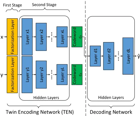
Figure 1: The architecture of the proposed TSLE paradigm. TEN is comprised of two networks, and each of which is a Two-Stage Label Embedding network: a factorization layer in the first stage; several hidden layers in the second stage. The decoding network includes a set of hidden layers.

proposed model contains two phases: a Twin Encoding Net-work projects instances and labels into a lower embedding space to get their codewords; a decoding network recovers label outputs from the codewords with a set of hidden layers.

Twin Encoding Network (TEN)

We present a novel neural network based encoding scheme. Since TSLE projects features and labels into a shared la-tent space, we introduce an architecture called Twin Encod-ing Network for encodEncod-ing process. Note that instances and labels have their own distribution. Therefore TEN uses a feature network and a label network which have a similar two-stage encoding architecture to produce codewords re-spectively. In what follows, we elaborate the feature network of TEN while the label network is under the same schema. Concretely, the feature network is comprised of two parts: a factorization layer and a set of hidden layers.

Factorization Layer In the first stage, the factorization layer maps each feature to a dense vector representation. Formally, we feed an instance vectorx= [x1, x2, ..., xp]T ∈ Rpinto the layer and then obtain a set of embedding vectors

Vemb = {v1x1,v2x2, ...,vpxp}wherevi ∈Rtis the

em-bedding parameter corresponding to thei-th feature. Then, we conduct a pairwise product of the embedding vectors, which can be regarded as a pooling operation since it does not involve extra parameters. Now we get a single vector g(x;V):

g(x;V) =

p

X

j=1 p

X

k=j+1

xjvjxkvk (5)

whereV = [v1,v2, ...,vp]∈Rt×pis the feature embedding

matrix, anddenotes element-wise product. This is the core operation of factorization layer that extracts second-order in-teractions between features.

However, the time complexity of Eq. (5) isO(tp2_{), which}

makes our model impractical when the inputs have a huge number of features or labels. To address this problem, we can reformulate Eq. (5) as:

g(x;V) =1 2[(

p

X

j=1

xjvj)2− p

X

j=1

(xjvj)2] (6)

wherev2_denotes_v_v_{. Now the pairwise product operation}

can be linearly computed inO(tp)time.

Moreover, owing to a sparse representation of inputs, which is common in real-world applications, we can only consider the embedding vectors for non-zero features, i.e.,Vemb = {vixi|xi 6= 0}. Consequently, the time

com-plexity is reduced toO(tpx), wherepxmay be a small

pos-itive integer that represents the average number of non-zero elements of each vector in the input matrix.

Notice that FM consists of two parts: a regression part and a pairwise factorization part. To generalize FM, the regres-sion part is not fed into the neural network in vanilla NFM, which limits its expressiveness. Hence, we combine the re-gression operation and the factorization operation in the first layer to sufficiently utilize the expressive ability of neural network:

Fac(x;V, A) =a0+ p

X

j=1

xjaj+g(x;V) (7)

where A = [a0,a1, ...,ap] ∈ Rt×(p+1) is the regression

parameter. To output a vector rather than a singular, we per-form multi-output regression which is different from the de-fault setting in vanilla NFM.

In contrast to other neural network based models (Yeh et al. 2017; Zhao et al. 2015) which learn high-order correla-tions directly, TSLE uses the factorization layer to extract second-order interactions between features and labels in ad-vance. Then we can efficiently learn higher-order correla-tions with deep neural network.

Hidden Layers Deep neural network has demonstrated its ability in learning representations from the raw data. The factorized vectors are then fed into a stack of fully con-nected layers to learn higher-order correlations in the second stage. Each layer can be customized to discover certain la-tent structures between features or labels. It is subjected to design and can be abstracted ascx=hE(Fac(x;V, A); Θx)

where hE denotes the hidden layers with parameters Θx.

cx ∈ Rd is the output codeword. In general, the input of

each layer is linearly transformed and then activated by a non-linear function,e.g., sigmoid, hyperbolic tangent (tanh) or Rectifier (ReLU).

Eventually, the last hidden layer outputs the codeword vectorcxwithout activation.

(4)

are distinct. Formally, the model can be expressed as follow:

cy=hE(Fac(y;U, B); Θy)

=hE(b0+ q

X

j=1

yjbj+g(y;U); Θy)

(8)

where cy ∈ Rd is the output codeword of labels. U =

[u1,u2, ...,uq] ∈ Rt×q and B = [b0,b1, ...,bq] ∈ Rt×(q+1)are the parameters of the label factorization layer.

Θyare the parameters of the hidden layers in the label

net-work.

Through such a twin architecture, we jointly encode the features and labels to the latent space.

Decoding Network

The decoding procedure recovers label outputyˆfrom code-wordcxwhich is the feature representation in latent space.

Traditionally, decoding is performed by maximizing a joint probability function (Zhang and Schneider 2011). Due to the requirement of solving a quadratic problem, such decoding technique is computationally expensive. To handle this prob-lem, we adapt the idea of (Yeh et al. 2017) and introduce a multi-layer decoding networkhD:

s1=σ1(Wd1cx+bd1)

s2=σ2(Wd2s1+bd2)

...

sL=σL(WdLsL−1+bdL)

ˆ

y=WoutsL+bout

(9)

wheresi,Wdi,bdi,σidenote the output vector, weight

ma-trix, bias vector and activation function for thei-th layer re-spectively.Wout andbout are the weight matrix and bias

vector for the last layer. By exploiting the inherent nonlin-earity of deep neural network, we can reconstruct our pre-dicted labels from the lower-dimensional codeword vector.

Training

Since our framework is comprised of two separate networks (an encoding network and a decoding network), the final ob-jective function can also be decomposed into two parts: a encoding loss and a decoding loss.

In encoding phase, inspired by (Zhang and Schneider 2012; Liu and Tsang 2015), a max margin formulation is involved such that the codeword is both discriminative and predictable. Define µ(i) = maxy∈N ei(i){||cxi −cyi||

2 2−

||cxi−cy|| 2

2+ ∆(yi,y)}, the encoding lossLEis designed

as follow:

LE=

1 N

N

X

i=1

max{0, µ(i)} (10)

For decoding, the goal is to reduce the prediction mistakes on unseen data. Among various choices of global error defi-nitions, we choose to adapt a popular label-correlation aware error function which is proposed by (Zhang and Zhou 2006):

LD=

1 N

N

X

i=1

1 |y1

i||y 0 i|

X

(e,g)∈y1

i×y0i

exp((ˆyi)g−(ˆyi)e)

(11)

Algorithm 1Training procedure of TSLE

Input: Feature matrix X, label matrix Y, learning rateη, leverage parametersλandα, dimension parametersd andt, size of nearest neighbork

Output: The optimal trainable parameters of TSLE 1: Compute the label set N ei(i)of instance xi for i =

1,2, ..., N

2: Initialize all trainable parameters with random values from Gaussian distribution

3: repeat

4: Randomly select a data samplexjandyj

5: Compute the output of the factorization layer F ac(xj;V, A), F ac(yj;U, B) and F ac(y;U, B)

wherey∈N ei(j)

6: Compute the codewordscxj,cyj andcy

7: Recover the output labelyˆjfromcxj

8: Compute the encoding lossLE by Eq. (10) and the

decoding lossLDby Eq. (11)

9: Compute the final lossLby Eq. (12)

10: Update all trainable parameters with Adam algorithm 11: untilConverge

Here,LD is the decoding loss. For thei-th instancexi,

y_i1is the set of the positive labels inyiandyi0is that of the

negative labels.| · |measures the cardinality of a set.(ˆyi)e

denotes thee-th entry of the predicted labelˆyi.

We note that existing label embedding approaches usually manipulate the encoding and decoding processes separately. To give our proposed model more robustness, the encoding and decoding losses are combined and leveraged by a posi-tive constantα. A regularization term is also added to pre-vent overfitting. Then the final lossLcan be formulated as:

L=LE+αLD+λ

X

φ∈Φ

||φ||2

(12)

whereΦdenotes the set of all parameters andλcontrols the regularization strength.||·||represents thel2norm of vectors

or the Frobenius norm of matrices.

We adapt Adam (Kingma and Ba 2014) instead of vanilla Stochastic Gradient Descent to iteratively update the pa-rameters with learning rate η. Adam has two main advan-tages: capability of dealing with sparse gradients and non-stationary objectives, and requiring little memory. Note that our proposed model is clearly defined, thus the computa-tional graphs (Fig. 1) can be easily built and the model can be straightly implemented using Machine Learning Toolkits like TensorFlow (Abadi et al. 2016) or Caffe (Jia et al. 2014). The pseudo code of TSLE is summarized in Algorithm 1.

Once the parameters are learnt, we can predict the label of a test inputˆxby roundingˆy=hD(cˆx).

Kernel View of TSLE

It is well-known that the theoretical properties of deep neural network are still not well understood. Therefore, we demon-strate a different view of TSLE for a better understanding.

(5)

any function that takes a matrix as input and outputs a vec-tor. Consequently, we can remove all the activation functions and biases. Then the hidden layers linearly project the em-bedding vectors into a latent space. Moreover, we preserve only two hidden layers in the feature network and one in the label network:

cx=Wx2W 1

xFac(x;V, A)

cy=Wy1Fac(y;U, B)

(13)

whereW1

x,Wx2 andWy1 are weight parameters. Here, we

setWx2 = Wy1. Comparing Eq. (4) with Eq. (13), we can

see that the specialised hidden layers project the embedding vectors in the same way as LM-kNN encodes the inputs.

Recall that a factorization layer is used to obtain the em-bedding vectors. While a recent work (Blondel et al. 2016) provides a kernel view of FM, our factorization layer actu-ally maps the original inputs into a polynomial kernel space. It is worth pointing that TEN and LM-kNN have similar ob-jective functions. Thus, if we regard the factorization layer as a preprocessing procedure of data, the specialised TSLE will have the same encoding phase as a kernelized LM-kNN, where the kernel function is exactly FM.

We have demonstrated the generalization ability of our proposed model. Furthermore, we show that TSLE has two main advantages. First, instead of linear projection, deep neural networks are used in encoding phase to better exploit high-order dependency. Second, TSLE is a typical margin-based algorithm and it is well-known that kernel trick can provide significant improvements for such algorithms. Since pairwise interactions commonly exist in multi-label datasets, FM will be a promising kernel function. Empirical study also proves that our proposed model outperforms LM-kNN.

Experiment

In this section, we evaluate the performance of our pro-posed TSLE and five state-of-the-art multi-label techniques on many real-world datasets over eight measurements. We conduct all experiments on a same workstation with an i7-5930K CPU, a TITAN Xp GPU and 64GB main memory running Linux platform.

Experimental Settings

Datasets We conduct experiments on seven real-world datasets from various domains.

• Cal500 (Turnbull et al. 2008): A music dataset containing human-generated musical annotations that describes 502 popular western musical tracks with 174 tags representing emotions, instruments, and other related concepts.

• Emotions (Trohidis et al. 2008): A music dataset consist-ing of hundreds of songs from 6 genres.

• Yeast (Elisseeff and Weston 2001): A biology dataset formed by micro-array expression data and phylogenetic profiles with 14 genes.

• Eurlex (Menc´ıa and F¨urnkranz 2008): A collection of documents about European Union law. Several EU-ROVOC descriptors, directory codes and subject matters

are available, corresponding to three individual datasets: Eurlex desc, Eurlex dc and Eurlex sm. Following the set-ting of (Zhang and Schneider 2012), we select the 10 most common labels to study.

• NUS-WIDE (Chua et al. 2009): A large-scale web image dataset with hundreds of thousands of instances that in-cludes 500-dimensional bag of words based on SIFT de-scriptions for 81 concepts.

More detailed information about the datasets can be found on the website1_.

Baselines We compare TSLE with several state-of-the-art multi-label classification approaches:

• BR (Tsoumakas, Katakis, and Vlahavas 2010): Binary Relevance predicts each label independently with a binary classifier. In this paper, we use neural network as the bi-nary classifier.

• ML-kNN (Zhang and Zhou 2007): Derived from the tra-ditionalk nearest neighbor algorithm, ML-kNN utilizes maximum a posteriori principle to determine the label set for the unseen instance.

• CPLST (Chen and Lin 2012): Based on minimizing an upper bound of the Hamming loss, CPLST combines the concepts of Principal Component Analysis (PCA) and Canonical Correlation Analysis (CCA) to improve PLST (Tai and Lin 2012) through the addition of feature infor-mation.

• LM-kNN (Liu and Tsang 2015): By linearly embedding features and labels into a low dimensional space, LM-kNN uses the Euclidean distance of instances in the latent space as a metric to findknearest neighbors and takes the weighted average of their labels as the predicted labels. • C2AE (Yeh et al. 2017): As the first deep neural network

based label embedding approach for multi-label classi-fication, C2AE integrates Deep Canonical Correlation Analysis (DCCA) (Reichart, Vulic, and Rotman 2018) and autoencoder to exploit label dependency.

Parameter Settings We implement our proposed TSLE based on TensorFlow. We randomly select 80% of the data for training and predict the labels with the rest 20%. The feature and label embedding matricesV andU are initial-ized with random values sampled from a standard Gaussian distribution. The dimension of embedding vectortis set to 256. BothhEandhDare composed of three fully connected

layers with ReLU as activation functions. The hidden di-mensions ofhEandhDare[64,64, d]and[d,64, q]

respec-tively, where d = min(32, q−1) is the dimension of the latent space. Each base classifier of BR is a neural network with dimensions of[64,64,1]. We setk= 3for ML-kNN, LM-kNN and our method. The default learning ratesηof all baselines (expect CPLST) and TSLE are10−3. The default leverage parameterαand regularization parameterλare set to1 and0.01 respectively. To test the stability of the pro-posed model, we also experiment TSLE on various learning rates ranging from10−4_to₅_×₁₀−3_{and different leverage}

1

(6)

Table 1: Results of Micro-F1 on all datasets (mean±standard deviation), the best ones are in bold.

Datasets BR ML-kNN CPLST LM-kNN C2AE TSLE

Cal500 0.3643±0.0153 0.3162±0.0146 0.3329±0.0064 0.3551±0.0092 0.4586±0.0011 0.4648±0.0088 Emotions 0.6047±0.0178 0.6585±0.0110 0.6430±0.0051 0.6152±0.0113 0.4563±0.0113 0.6933±0.0040 Yeast 0.4037±0.0042 0.6262±0.0142 0.4670±0.0051 0.5365±0.0098 0.5459±0.0099 0.5908±0.0068 Eurlex desc 0.3605±0.0093 0.6584±0.0061 0.3173±0.0106 0.7050±0.0122 0.3671±0.0146 0.7057±0.0032 Eurlex dc 0.5455±0.0117 0.9193±0.0063 0.4928±0.0193 0.9206±0.0059 0.4091±0.0146 0.9492±0.0098 Eurlex sm 0.4155±0.0070 0.8177±0.0059 0.5897±0.0194 0.8046±0.0070 0.3583±0.0070 0.8230±0.0060 NUS-WIDE 0.2356±0.0053 0.1781±0.0102 0.2236±0.0036 0.2751±0.0029 0.3685±0.0044 0.3815±0.0098

Table 2: Results of Macro-F1 on all datasets (mean±standard deviation), the best ones are in bold.

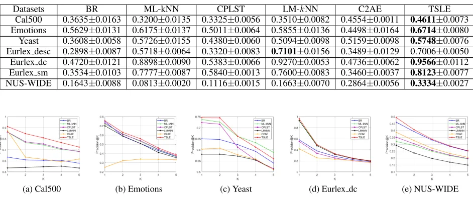
Table 3: Results of Example-F1 on all datasets (mean±standard deviation), the best ones are in bold.

(a) Cal500 (b) Emotions (c) Yeast (d) Eurlex dc (e) NUS-WIDE

Figure 2: Precision@Kof all methods on various datasets.

parameters ranging from0.3 to3. Other parameters in the baselines are set to their default values.

Measurements To better measure the performance, we adapt several widely-used metrics:

• Micro-F1: It calculates true positives/negatives and false positives/negatives over labels, and then computes an overall F-measure.

• Macro-F1: It is the unweighted mean of label F-measure.

• Example-F1: It is the unweighted mean of instance F-measure.

• Precision@K: It is the proportion of labels in the Top-K set that are correctly predicted.

Experimental Results

Prediction Performance Table 1, 2 and 3 list the Micro-F1, Macro-F1 and Example-F1 results of baselines and our model in respect of different datasets. Fig. 2 shows the Precision@K results on different datasets where the rank-ing positionKranges from 1 to 5. From the results, we can tell that:

(7)

po-(a) Micro-F1 (b) Macro-F1

Figure 3: Micro-F1 and Macro-F1 of TSLEw.r.t. different learning rates (η)

(a) Micro-F1 (b) Macro-F1

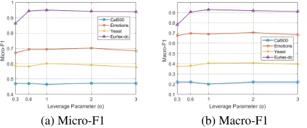
Figure 4: Micro-F1 and Macro-F1 of TSLEw.r.t. different leverage parameters (α)

sitions. These results demonstrate that TSLE achieves su-perior performance than those baselines.

• BR and ML-kNN underperform LM-kNN and TSLE over many measurements. Therefore, exploiting label correla-tions can notably improve the prediction performance.

• CPLST is much inferior to C2AE, LM-kNN and TSLE. With simple linear projection, CPLST cannot effectively explore the latent label spaces.

• It is worth pointing that C2AE works well on many datasets, which proofs that deep neural network can ef-ficiently extract high-order label correlations. However, since its criterion does not optimize the discriminability of the codewords, it is unstable and sensitive to noisy data. Moreover, C2AE ignores the difficulty of learning high-order label correlations directly due to the sparsity of la-bels, and thus underperforms TSLE.

• LM-kNN and TSLE are the most successful methods on all datasets. However, TSLE is better for two reasons. First, a factorization layer, which works well under sparse setting, is used as a kernel function to learn pairwise cor-relations in advance. Second, DNN can efficiently exploit higher-order label dependency and effectively recover the output labels from codewords.

Parameter Sensitivity In this section, we explore the hy-perparameter sensitivity of our model to find out the strength and relevance of the inputs in determining the variation in the output. Fig. 3 reports Micro-F1 and Macro-F1 results un-der different learning ratesηon four datasets. Fig. 4 shows

the same measurements under different loss leverage param-etersα. The experimental results fluctuate lightly according to different orders of magnitude, but they are substantially robust within an acceptable range. In conclusion, the above results assure the quality and stability of TSLE.

Conclusion

To handle complicated label hierarchies, this paper proposes a novel Two-Stage Label Embedding (TSLE) paradigm for MLC. Based on NFM (He and Chua 2017), a Twin Encoding Network is introduced to jointly embed features and labels into a latent space. In the first stage, a factorization layer extracts pairwise feature and label interactions. Then a set of hidden layers is applied to learn higher-order correlations in the second stage. Inspired by (Yeh et al. 2017), we use deep neural network to recover the output labels from the codewords of instances in decoding phase. To give TSLE more robustness, the final objective function is leveraged between two parts: a max margin formulated encoding loss for discriminative and predictable codewords, and a label-correlation aware decoding loss. Furthermore, a regulariza-tion term is also added to alleviate overfitting. For a better understanding, we provide a kernel insight to show the gen-eralization ability of TSLE. In the experiments, we demon-strate that our TSLE notably outperforms other state-of-the-art methods with quality assurance.

Acknowledgments

This research is supported by National Key Research and Development Program (2017YFB1201001).

References

Abadi, M.; Barham, P.; Chen, J.; Chen, Z.; Davis, A.; Dean, J.; Devin, M.; Ghemawat, S.; Irving, G.; Isard, M.; Kudlur, M.; Levenberg, J.; Monga, R.; Moore, S.; Murray, D. G.; Steiner, B.; Tucker, P. A.; Vasudevan, V.; Warden, P.; Wicke, M.; Yu, Y.; and Zheng, X. 2016. Tensorflow: A system for large-scale machine learning. In12th USENIX Symposium on Operating

Systems Design and Implementation, 265–283.

Blondel, M.; Ishihata, M.; Fujino, A.; and Ueda, N. 2016. Polynomial networks and factorization machines: New in-sights and efficient training algorithms. InICML, 850–858. Cao, B.; Zhou, H.; Li, G.; and Yu, P. S. 2016. Multi-view ma-chines. InProceedings of the Ninth ACM International

Con-ference on Web Search and Data Mining, 427–436. ACM.

Chen, Y.-N., and Lin, H.-T. 2012. Feature-aware label space dimension reduction for multi-label classification. In NIPS, 1538–1546.

Chua, T.-S.; Tang, J.; Hong, R.; Li, H.; Luo, Z.; and Zheng, Y.-T. 2009. Nus-wide: A real-world web image database from national university of singapore. In Proc. of ACM Conf. on

Image and Video Retrieval (CIVR’09).

Deng, C.; Chen, Z.; Liu, X.; Gao, X.; and Tao, D. 2018a. Triplet-based deep hashing network for cross-modal retrieval.

IEEE Transactions on Image Processing27(8):3893–3903.

(8)

Elisseeff, A., and Weston, J. 2001. A kernel method for multi-labelled classification. InNIPS, 681–687.

Gong, C.; Liu, T.; Tao, D.; Fu, K.; Tu, E.; and Yang, J. 2015. Deformed graph laplacian for semisupervised learning.

IEEE transactions on neural networks and learning systems

26(10):2261–2274.

Gong, C.; Tao, D.; Maybank, S. J.; Liu, W.; Kang, G.; and Yang, J. 2016. Multi-modal curriculum learning for semi-supervised image classification. IEEE Transactions on Image

Processing25(7):3249–3260.

He, X., and Chua, T.-S. 2017. Neural factorization machines for sparse predictive analytics. InProceedings of the 40th In-ternational ACM SIGIR conference on Research and

Develop-ment in Information Retrieval, 355–364.

Hsu, D.; Kakade, S.; Langford, J.; and Zhang, T. 2009. Multi-label prediction via compressed sensing. InNIPS, 772–780. Jia, Y.; Shelhamer, E.; Donahue, J.; Karayev, S.; Long, J.; Gir-shick, R. B.; Guadarrama, S.; and Darrell, T. 2014. Caffe: Convolutional architecture for fast feature embedding. In

Pro-ceedings of the ACM International Conference on Multimedia,

675–678.

Kingma, D. P., and Ba, J. 2014. Adam: A method for stochas-tic optimization.CoRRabs/1412.6980.

Liu, W., and Tsang, I. W. 2015. Large margin metric learning for multi-label prediction. InAAAI, 2800–2806.

Liu, W., and Tsang, I. W. 2017. Making decision trees feasi-ble in ultrahigh feature and label dimensions. The Journal of

Machine Learning Research18(1):2814–2849.

Liu, W.; Xu, D.; Tsang, I.; and Zhang, W. 2018. Metric learning for multi-output tasks.IEEE Transactions on Pattern

Analysis and Machine Intelligence.

Liu, W.; Tsang, I. W.; and M¨uller, K.-R. 2017. An easy-to-hard learning paradigm for multiple classes and multiple la-bels.The Journal of Machine Learning Research18(1):3300– 3337.

Menc´ıa, E. L., and F¨urnkranz, J. 2008. Efficient pairwise multilabel classification for large-scale problems in the legal domain. InECML/PKDD, 50–65.

Nam, J.; Loza Menc´ıa, E.; Kim, H. J.; and F¨urnkranz, J. 2017. Maximizing subset accuracy with recurrent neural networks in multi-label classification. InNIPS, 5419–5429.

Read, J.; Pfahringer, B.; Holmes, G.; and Frank, E. 2011. Clas-sifier chains for multi-label classification. Machine Learning

85(3):333–359.

Reichart, R.; Vulic, I.; and Rotman, G. 2018. Bridging lan-guages through images with deep partial canonical correlation analysis. InACL, 910–921.

Rendle, S. 2012. Factorization machines with libfm. ACM Transactions on Intelligent Systems and Technology (TIST)

3(3):57.

Schapire, R. E., and Singer, Y. 2000. Boostexter: A boosting-based system for text categorization. Machine Learning

39(2/3):135–168.

Tai, F., and Lin, H.-T. 2012. Multilabel classification with principal label space transformation. Neural Computation

24(9):2508–2542.

Trohidis, K.; Tsoumakas, G.; Kalliris, G.; and Vlahavas, I. P. 2008. Multi-label classification of music into emotions. In

ISMIR, volume 8, 325–330.

Tsoumakas, G.; Katakis, I.; and Vlahavas, I. 2010. Mining multi-label data. InData Mining and Knowledge Discovery

Handbook. 667–685.

Turnbull, D.; Barrington, L.; Torres, D. A.; and Lanckriet, G. R. G. 2008. Semantic annotation and retrieval of music and sound effects. IEEE Trans. Audio, Speech & Language

Pro-cessing16(2):467–476.

Wang, J.; Yang, Y.; Mao, J.; Huang, Z.; Huang, C.; and Xu, W. 2016. CNN-RNN: A unified framework for multi-label image classification. InCVPR, 2285–2294.

Yang, E.; Deng, C.; Li, C.; Liu, W.; Li, J.; and Tao, D. 2018. Shared predictive cross-modal deep quantization.IEEE

Trans-actions on Neural Networks and Learning Systems(99):1–12.

Yeh, C.-K.; Wu, W.-C.; Ko, W.-J.; and Wang, Y.-C. F. 2017. Learning deep latent space for multi-label classification. In

AAAI, 2838–2844.

Zhang, Y., and Schneider, J. G. 2011. Multi-label output codes using canonical correlation analysis. InAISTATS, 873–882. Zhang, Y., and Schneider, J. G. 2012. Maximum margin out-put coding. InICML.

Zhang, M., and Zhou, Z. 2006. Multi-label neural networks with applications to functional genomics and text categoriza-tion. IEEE Trans. Knowl. Data Eng.18(10):1338–1351. Zhang, M.-L., and Zhou, Z.-H. 2007. Ml-knn: A lazy learn-ing approach to multi-label learnlearn-ing. Pattern Recognition

40(7):2038–2048.