Learning by Unsupervised Nonlinear Diffusion
Mauro Maggioni [email protected]
Department of Mathematics, Department of Applied Mathematics and Statistics,
Mathematical Institute of Data Sciences, Institute of Data Intensive Engineering and Sci-ence,
Johns Hopkins University, Baltimore, MD 21218, USA
James M. Murphy [email protected]
Department of Mathematics
Tufts University, Medford, MA 02155, USA
Editor: Aapo Hyv¨arinen
Abstract
This paper proposes and analyzes a novel clustering algorithm, called learning by unsupervised nonlinear diffusion (LUND), that combines graph-based diffusion ge-ometry with techniques based on density and mode estimation. LUND is suitable for data generated from mixtures of distributions with densities that are both mul-timodal and supported near nonlinear sets. A crucial aspect of this algorithm is the use of time of a data-adapted diffusion process, and associated diffusion distances, as a scale parameter that is different from the local spatial scale parameter used in many clustering algorithms. We prove estimates for the behavior of diffusion distances with respect to this time parameter under a flexible nonparametric data model, identifying a range of times in which the mesoscopic equilibria of the un-derlying process are revealed, corresponding to a gap between within-cluster and between-cluster diffusion distances. These structures may be missed by the top eigenvectors of the graph Laplacian, commonly used in spectral clustering. This analysis is leveraged to prove sufficient conditions guaranteeing the accuracy of LUND. We implement LUND and confirm its theoretical properties on illustrative data sets, demonstrating its theoretical and empirical advantages over both spectral and density-based clustering.
Keywords: unsupervised learning, clustering, spectral graph theory, manifold learning, diffusion geometry
1. Introduction
Unsupervised learning is a central problem in machine learning, requiring that data be analyzed without a priori knowledge of any class labels. A common unsupervised problem is clustering, in which the data is to be partitioned into clusters so that each
c
cluster contains similar points and distinct clusters are sufficiently separated. Even with suitable definitions of “similarity” and “separation”, this problem is typically ill-posed, requiring various geometric, analytic, topological, and statistical assumptions on the data and measurement method be imposed to make it tractable. Feature extraction is often combined with these standard methods (e.g. K-means) to improve clustering performance.
In particular,spectral methods construct graphs representing data, and use the spec-tral properties of the resulting graph Laplacian to produce structure-revealing fea-tures in the data. Graphs often encode pairwise similarities between points, typi-cally at a local “spatial” scale, often determined by a parameter σ. For example only points xi, xj within distance 4σ of each other may be connected, with weight
exp(−kxi−xjk22/σ2). From the graph, global features on the data may be derived, for example by considering the eigenfunctions of the random walk on the graph. Alternatively, graphs may be used to introduce data-adaptive distances, such as
dif-fusion distances, which are associated to random walks and diffusion processes on
graphs. Diffusion distances do not depend only on the graph itself, but also on a time parameter t that determines a scale on the graph at which these distances are considered, related to the time of diffusion or random walk. Choosing σ in graph-based algorithms, and both σ and t in the case of diffusion distances, is important in both theory and applications. However, their role is well-understood only in certain regimes (e.g. asymptotically for σ, t → 0+) which are of interest in some problems (e.g. manifold learning) but not necessarily for clustering.x
We propose the Learning by Unsupervised Nonlinear Diffusion (LUND) scheme for clustering, which combines diffusion distances and density estimation to efficiently cluster data generated from a nonparametric model. At the same time, we advance the understanding of the relationship between the local “spatial” scale parameter σ
and the diffusion time parameter t in the context of clustering, demonstrating how the role of t can be exploited to successfully cluster data sets for which K-means, spectral clustering, or density-based clustering methods fail. We provide quantitative bounds and guarantees on the performance of the proposed clustering algorithm for data that may be highly nonlinear (i.e. non-convex, elongated, ellipsoidal, etc.) and of variable density.
1.1 Major Contributions and Outline
This article makes two major contributions. First, explicit estimates on diffusion
distances for nonparametric clustered data are proved: we obtain lower bounds for
data” of the diffusion distances, is very different from the commonly-used scaling parameterσ in the construction of the underlying graph, which is a local spatial scale measured in the ambient space. Relationships betweent andσare well-understood in the asymptotic case ofn→+∞,σ→0+ (at an appropriate rate withn; see Coifman et al. (2005), Lafon et al. (2006), and Von Luxburg (2007)) and t → 0+ (essentially Varadhan’s lemma applied to diffusions on a manifold; see Den Hollander (2008), Jones et al. (2008), and references therein). These asymptotic relationships at small scales imply that the choice oft is essentially irrelevant, since in these limits diffusion distances are essentially geodesic distances. However, the clustering phenomena we are interested in are far from this regime, and we show that the interplay between t,
σ, andn becomes crucial.
Second, the LUND clustering scheme is proposed and shown to enjoy performance guarantees for clustering of certain non-parametric mixture models. We prove suffi-cient conditions for LUND to correctly determine the number of clusters in the data and to have low clustering error. Computationally, we present an efficient algorithm implementing LUND, which scales near-linearly in the number of points n, in the ambient dimension D, and exponentially in the intrinsic dimension of the data. We verify the properties of the LUND scheme and algorithm on synthetic data, studying the relationships between the different parameters in LUND, in particular between
σ and t, and compare with popular and related the graph-based spectral clustering
and fast search and find of density peaks clustering (FSFDPC) (Rodriguez and Laio,
2014) algorithms, illustrating weaknesses of these methods and corresponding advan-tages of LUND. LUND may be understood as a combination of these two methods, in that it integrates diffusion distances (which are graph-based) and an outlier ro-bustness procedure into the FSFDPC framework, which uses Euclidean distances. Indeed, our experiments illustrate how LUND combines the benefits of graph-based and density-based methods.
The outline of the article is as follows. Background is presented in Section 2. In Section 3, motivational data sets and a summary of the theoretical results are pre-sented and discussed. Theoretical comparisons with related clustering methods are also made in Section 3. Estimates on diffusion distances are proved in Section 4. Performance guarantees for the LUND algorithm are proved in Section 5. Numerical experiments and computational complexity are discussed in Section 6. Conclusions and future research directions are given in Section 7.
2. Background
2.1 Background on Clustering
2.1.1 K-Means
A classical and popular clustering algorithm isK-means (Steinhaus, 1957; Friedman et al., 2001) and its variants (Ostrovsky et al., 2006; Arthur and Vassilvitskii, 2007; Park and Jun, 2009), which is often used in conjunction with feature extraction methods. K-means partitions the data intoK (a parameter) groups,{Ck}Kk=1, chosen to minimize within-cluster dissimilarity: C∗ = arg min{Ck}Kk=1
PK
k=1
P
x∈Ckkx−x¯kk
2 2, where ¯xkis the mean of thekthcluster (for a given partition, it is the minimizer of the
least squares cost in the inner sum). While popular, K-means and its variants may perform poorly for data sets that are not the union of well-separated, near-spherical clusters, and are sensitive to outliers.
2.1.2 Hierarchical Clustering Methods
Hierarchical methods iteratively merge or split clusters in order to produce a mul-tiscale family of partitions known as a dendrogram (Friedman et al., 2001). More precisely, a dendrogram for n data points is a family of clusterings {Ci}ni=1 such that
C1 is the clustering of n singleton clusters, and Ci is related to Ci+1 in that the two clusters minimizing some linkage function in Ci are merged in Ci+1. Single linkage
clustering (SLC) (Sneath, 1957; Gower and Ross, 1969; Friedman et al., 2001) is a
particular hierarchical clustering method that iteratively merges clusters according to the linkage function LSLC(C1, C2) = minx1∈C1,x2∈C2kx1−x2k2; metrics other than
the `2 norm may be used. For clusters that are well-separated, single linkage cluster-ing is known to perform well (Arias-Castro, 2011), despite lack of strong statistical consistency in dimensions greater than 1 (Hartigan, 1981).
2.1.3 Density and Mode-Based Methods
Density and mode-based clustering methods detect regions of high-density and low-density to determine clusters. The DBSCAN (Ester et al., 1996) and DBCLASD
(Xu et al., 1998) algorithms assign to the same cluster points that are close and have many near neighbors, and flag as outliers points that lie alone in low-density regions.
The mean-shift algorithm and variants (Fukunaga and Hostetler, 1975; Comaniciu
and Meer, 2002; Chac´on, 2012; Genovese et al., 2016) push points towards regions of high-density, and associate clusters with these high-density points, sometimes called
modes. Both DBSCAN and mean-shift clustering suffer from a lack of robustness to
outliers and depend strongly on parameter choices.
The fast search and find of density peaks clustering algorithm (FSFDPC) (Rodriguez
strong geometric and statistical assumptions on the data are satisfied. The main reason is that Euclidean distances are used to find modes, which is inappropriate for data drawn from mixtures of distributions supported near nonlinear sets (see, for example, Figure 18). Moreover, FSFDPC is not robust to outliers, which may be far from other points but be of low-density.
2.1.4 Spectral Methods
Spectral clustering methods compute features that reveal the structure of data that
may deviate from the spherical, Gaussian shapes ideal forK-means, and in particular may be nonlinear or elongated in shape. This is done by building local connectivity graphs on the data that encode pairwise similarities between points, then computing a spectral decomposition of adjacency or random walk or Laplacian operators defined on this graph.
Let X = {xi}in=1 ⊂ RD be a set of points to cluster. Let G be a graph with vertices corresponding to points of X and edges stored in an n × n symmetric weight matrix W. Often one chooses Wij = K(xi, xj) for some (symmetric,
of-ten radial and rapidly decaying) nonnegative kernel K : RD ×
RD → R, such as
K(xi, xj) = exp(−||xi −xj||2/σ2) for some choice of scaling parameter σ > 0. The
graphG may be fully connected, or it may be a nearest neighbors graph with respect to some metric. LetDbe the diagonal matrixDii :=
Pn
j=1Wij. Thegraph Laplacian
is constructed as L=D−W. One then normalizes L to acquire either the random
walk Laplacian LRW = D−1L = I−D−1W or the symmetric normalized Laplacian
LSYM = D−
1 2 L D−
1
2 = I−D− 1 2WD−
1
2. We focus on LSYM in what follows. It can
be shown that LSYM has real eigenvalues 0 = λ1 ≤ · · · ≤ λn ≤ 2 and corresponding
eigenvectors {φi}ni=1. The original data X can be clustered by clustering the em-bedded data xi 7→ (φ1(xi), φ2(xi), . . . , φM(xi)) for an appropriate choice of M ≤ n.
In this step typically K-means is used, though Gaussian mixture models may (and perhaps should) be used, as they enjoy, unlikeK-means, a suitably-defined statistical consistency guarantee in the infinite sample limit (Athreya et al., 2017).
Spectral clustering relaxes a graph-cut problem: for a collection of subsetsX1, . . . , XK ⊂ X, the correspondingnormalized cutis Ncut(X1, . . . , XK) = PKk=1cut(Xk, Xkc)/vol(Xk),where
cut(A, B) = P
xi∈A,xj∈BWij, vol(A) =
P
xi∈A
Pn
j=1Wij. Minimizing Ncut yields
clusters that are simultaneously separated and balanced (Shi and Malik, 2000). This NP-hard problem may be relaxed by analyzing the first K eigenvectors of LSYM (Shi and Malik, 2000; Ng et al., 2002), or via a semidefinite programming problem (Ling and Strohmer, 2018).
Weaknesses of spectral clustering were scrutinized by Nadler and Galun (2007). They show the top eigenvectors of the random walk matrix P—defined on{xi}ni=1 sampled fromp(x) proportional toe−U(x)/2 for some potential function U(x)—converge under a suitable scaling as n→ ∞ to the top eigenfunctions of the Fokker-Planck operator
-14 -12 -10 -8 -6 -4 -2 0 2 -6 -4 -2 0 2 4 6
(a) Data to Cluster (Nadler and Galun, 2007)
-14 -12 -10 -8 -6 -4 -2 0 2 -6 -4 -2 0 2 4 6
(b) Spectral clustering (Shi and Malik, 2000)
-14 -12 -10 -8 -6 -4 -2 0 2 -6 -4 -2 0 2 4 6
(c) Spectral clustering (Ng et al., 2002)
-16 -14 -12 -10 -8 -6 -4 -2 0 2 4 -8 -6 -4 -2 0 2 4 6 8
(d) Eigenvector 2
-16 -14 -12 -10 -8 -6 -4 -2 0 2 4 -8 -6 -4 -2 0 2 4 6 8
(e) Eigenvector 3
-16 -14 -12 -10 -8 -6 -4 -2 0 2 4 -8 -6 -4 -2 0 2 4 6 8
(f) Eigenvector 4
-16 -14 -12 -10 -8 -6 -4 -2 0 2 4 -8 -6 -4 -2 0 2 4 6 8
(g) Eigenvector 5
-16 -14 -12 -10 -8 -6 -4 -2 0 2 4 -8 -6 -4 -2 0 2 4 6 8
(h) Eigenvector 6
Figure 1: In (a), three Gaussians of essentially the same density are shown. Results of spectral clustering are shown in (b) (Shi and Malik, 2000) and (c) (Ng et al., 2002). In (d) - (h), the first five non-trivial eigenvectors are shown. As noted by Nadler and Galun (2007), the underlying density for this data yields a Fokker-Planck operator whose low-energy eigenfunctions cannot distinguish between the two smaller clusters, thus preventing spectral clustering from succeeding: higher energy eigenfunctions are required. For this example, the sixth non-trivial eigenvector localizes sufficiently on the small clusters to allow for correct determination of the cluster structure; this eigenvector is not used in traditional spectral clustering algorithms.
the structure of the leading eigenfunctions ofL (Gardiner, 2009): they correspond to the time scales of the slowest transitions between different clusters and the equilibrium times within clusters. The relationships between these quantities determine which eigenfunctions ofL(orP) reveal the cluster structure in the data. Gavish and Nadler (2013) further analyze related connections between normalized cuts and cluster exit times. Nadler and Galun (2007) present data which cannot be clustered with spectral clustering (Shi and Malik, 2000; Ng et al., 2002); see Figure 1.
2.2 Background on Diffusion Distances
One of the primary tools in the proposed clustering algorithm is diffusion distances, a class of data-dependent distances computed by constructing Markov processes on data that capture its intrinsic structure (Coifman et al., 2005; Coifman and Lafon, 2006; Lafon et al., 2006; Coifman et al., 2008; Singer and Coifman, 2008; Rohrdanz et al., 2011; Zheng et al., 2011; Lederman and Talmon, 2018; Lederman et al., 2015; Czaja et al., 2016; Li et al., 2017). We consider diffusion on the point cloud X =
{xi}ni=1 ⊂RD via a Markov chain (Levin et al., 2009) with state spaceX. LetPbe the correspondingn×ntransition matrix. The following shall be referred to as the usual
assumptions on P: P is reversible, irreducible, aperiodic, and therefore ergodic. A
j for some appropriate scale parameter σ ∈ (0,∞). The parameter σ encodes the interaction radius of each point: σ large allows for long-range interactions between points that are `2-far, while σ small allows only for short-range interactions. Then P = D−1W, where D is the diagonal degree matrix with Dii =
Pn
`=1Wij. This1
row-normalizes P: Pn
j=1Pij = 1, ∀i = 1, . . . , n. Since it is ergodic, P has a unique
stationary distribution π satisfying πP=π, given by πi =Dii/
Pn
j=1Djj.
Diffusion processes on graphs lead to a data-dependent notion of distance, known
as diffusion distance (Coifman et al., 2005; Coifman and Lafon, 2006). While the
focus of the construction is on diffusion distances and the diffusion process itself, we mention that diffusion maps provide a way of efficiently computing and visual-izing large-time diffusion distances in Euclidean space, and at the same time may be understood as a type of nonlinear dimension reduction, in which data in a high number of dimensions may be embedded in a low-dimensional space by a nonlinear coordinate transformation. In this regard, diffusion maps are related to nonlinear dimension reduction techniques such as Isomap (Tenenbaum et al., 2000), Laplacian eigenmaps (Belkin and Niyogi, 2003), and local linear embedding (Roweis and Saul, 2000), kernel PCA (with a data-adapted kernel), among many others.
Definition 2.1 LetX ={xi}in=1 ⊂RD and letPbe a Markov process onXsatisfying
the usual assumptions and with stationary distribution π. Let π0 be a probability
distribution on X. For points xi, xj ∈ X, let pt(xi, xj) = (Pt)ij, for some t∈[0,∞).
The diffusion distance at time t between x, y ∈X is defined, for ν =π0/π, by
Dt(x, y) =
s X
u∈X
(pt(x, u)−pt(y, u))2ν(u) =||pt(x,·)−pt(y,·)||`2(ν).
If the underlying graph is generated from data sampled from a low-dimensional man-ifold, then diffusion distance parametrizes this low-dimensional structure (Coifman et al., 2005; Jones et al., 2008; Singer et al., 2009; Singer and Wu, 2012, 2016; Talmon and Wu, 2018). Indeed, diffusion distances admit a formulation in terms of the (right) eigenfunctions of P:
Dt(x, y) =
v u u t
n
X
`=1
λ2t
` (ψ`(x)−ψ`(y))2, (2.2)
where{(ψ`, λ`)}n`=1 are the right eigenpairs ofP, ordered so that 1 =λ1 > λ2 ≥λ3 ≥
· · · ≥λn >−1, and noting that ψ1 is constant by construction.
Diffusion distances are parametrized by t, which measures how long the diffusion process on G has run. Small t allows a small amount of diffusion, which may prevent the interesting geometry of X from being discovered, but provides detailed, fine scale
1. Note that with some abuse of notation we denote the entries ofPbyPij, reserving the notation
information. Large t allows the diffusion process to run for so long that the fine geometry may be washed out, leaving only coarse scale information. We will relate properties of clustered data X tot.
3. Data Model and Overview of Main Results
Among the main results of this article are sufficient conditions for clustering certain discrete data X ⊂ RD. The data X is modeled as a realization from a probability
distribution
µ=
K
X
k=1
wkµk, wk≥0,
K
X
k=1
wk = 1, (3.1)
where each µk is a probability measure. Intuitively, our results require separation
and cohesion conditions on {µk}Kk=1. That is, each µk is far from µk0, k 6= k0 and
connections are strong (in a suitable sense) within each µk. X ={xi}ni=1 is generated by drawing, for each i, one of the K clusters, say ki, according to the multinomial
distribution with parameters (w1, . . . , wK), and then drawingxifromµki. The clusters in the data are defined as the subsets ofXwhose samples were drawn from a particular
µk, that is, we define the cluster Xk := {xi ∈ X : ki = k}. Given X, the goal of
clustering is to estimate these Xk, and to estimate K. Throughout the theoretical
analysis of this article, we will define the accuracy of a set of labels {Yi}ni=1, Yi ∈
{1, . . . , K}, learned from an unsupervised algorithm to be |{i | Yi =ki}|/n, i.e. the
proportion of points correctly labeled.
The model (3.1) is nonparametric and makes few explicit assumptions onµ. We will allowµkto be supported near a non-linear set (e.g. a nonconvex subset, or a
subman-ifold in RD) and be multimodal (i.e. with multiple high-density regions). These
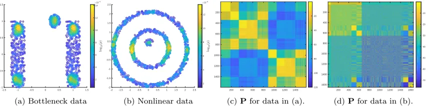
fea-tures may cause prominent clustering methods to fail, e.g. K-means, which requires near-spherical or well-separated clusters (Dasgupta and Schulman, 2007; Mixon et al., 2017); Gaussian mixture models, which handle well spherical and ellipsoidal clusters, but may struggle with clusters exhibiting different, non-elliptical geometries (for ex-ample those shown in Figure 2 (b)); spectral clustering, which can fail for highly elongated clusters or clusters of different sizes and densities; density-based methods, which are sensitive to noise and clusters of very different densities, and may require care in setting parameters or implementing adaptive parameters. Two simple, mo-tivating examples are in Figure 2. They feature variable densities, variable levels of connectivity, both within and across clusters, and (for the second example) nonlinear cluster shapes.
-1.5 -1 -0.5 0 0.5 1 1.5 -1 -0.5 0 0.5 1 1.5 2 4 6 8 10 12 14 10-4
(a) Bottleneck data
-2 -1.5 -1 -0.5 0 0.5 1 1.5 2 2.5 -2 -1.5 -1 -0.5 0 0.5 1 1.5 2 2.5 2 4 6 8 10 12 10-4
(b) Nonlinear data
200 400 600 800 1000 1200 1400 200 400 600 800 1000 1200 1400 -120 -100 -80 -60 -40 -20
(c)Pfor data in (a).
200 400 600 800 1000 1200 1400 1600 200 400 600 800 1000 1200 1400 1600 -70 -60 -50 -40 -30 -20 -10
(d)Pfor data in (b).
Figure 2: Subfigures (a) and (b) show two data sets—linear and nonlinear—colored by log10(p(x)), where p(x) is the empirical density. In (c), (d), we show the corresponding Markov transition ma-tricesP, with entry magnitudes shown in log10 scale. We sorted the rows and columns so that the
structure in these matrices become apparent (of course, the algorithms are independent of the sort-ing). The Markov chains are ergodic, but close to being reducible. Indeed, these transition matrices show hierarchical structure, with large within-cluster transitions and uniformly small probabilities of transition between clusters. The analysis of Section 4 makes this intuition precise. The transition matrices were constructed using the Gaussian kernel as in Section 2.2, with Euclidean distances and
σ=.25
3.1 Summary of Main Results
Our first result shows that the within-cluster and between-cluster diffusion distances can be controlled, as soon asPtis approximately block constant in some sense. Define
the (worst-case) within-cluster and between-cluster diffusion distances as:
Dtin= max
k x,ymax∈Xk
Dt(x, y), Dtbtw= min
k6=k0x∈Xmin
k,y∈Xk0
Dt(x, y). (3.2)
Our results guarantee thatDint is small andDbtwt is large in terms of a constant , for allt in some time intervalT. The intervalT depends on both data-driven quantities of the matrixP(which may be understood as geometrically intrinsic to the underlying cluster structure), as well as . This simplification of Theorem 4.12 holds:
Theorem 3.3 Let X = SK
k=1Xk and let P be a corresponding Markov transition
matrix onX, inducing diffusion distancesDt. Then there exist non-negative constants
{Ci}5i=1 such that the following holds: for any >0 we have
C1ln
C2
< t < C3 =⇒ Dtin ≤C4, Dbtwt ≥C5−C4.
The constants {Ci}5i=1 are defined precisely in Section 4, but to get a sense of them, letS be an idealized version ofPin which all edges between clusters are deleted and redirected back into the cluster; this will be made precise by the notion of stochastic complement in Definition 4.7. Let S∞ be a block diagonal matrix consisting of K
rank 1 blocks, corresponding to the equilibrium transition matrices of the the blocks of S. The constants {Ci}5i=1 may be interpreted as follows:
• C1, C2 are related to the compactness or irreducibility of the clusters Xk, in
diagonal block corresponding to a cluster, then C1 = 0 and C2 = O(1), inde-pendently ofn.
• C3 is related to the transition probabilities between clusters in P. In the ide-alized case that there are no transitions between any of the clusters, C3 =∞. More generally, if the probabilities of transitions between clusters are small, then C3 will be large.
• C4 is related to the balance of S∞ relative to P. If each row of S∞− P is constant, then C4 = 1/
√
n.
• C5 is related to how balanced the equilibrium distributions are on each cluster. IfS∞ is block constant with blocks of the same size, thenC5 = 1/
√
n.
The time interval T := [C1ln C2
, C3] depends on , and there is tension in the role of between the condition t ∈ T and the conclusion that Din
t ≤ C4, Dbtwt ≥
C5−C4. For large ,T may be quite wide, but the conclusion on diffusion distances is weak (or even trivial if > C5/C4). On the other hand, small induces strong separation between within-cluster diffusion distances and between-cluster diffusion distances, at the expense of shrinking T. Indeed, for 0 < C1, C2, C3 < ∞ fixed, T shrinks to the empty set as →0+.
Suppose indeed that the each cluster is compact (C1 small, C2 =O(1)), the clusters are well-separated (C3 large), and balanced in the sense that S∞−Pis constant and S∞ is block-constant with blocks of the same size (C4 =C5 = 1/
√
n). Then for >0,
t ∈
C1ln
C2
, C3
=⇒ D
btw
t
Din
t
≥ C5−C4
C4
=O
1
,
which suggests strong separation with diffusion distances independently of n when
is small. In particular, as the clusters become more separated (C3 increases) the time interval on which theDbtw
t /Dtinremains large widens on the right. Similarly, the
more compact or irreducible the clusters become (C1 becomes smaller), the wider the interval becomes on the left. In the ideal case that C1 = 0 (clusters are localized at single points),C3 =∞(infinite separation between clusters), the ratioDtbtw/Dint =∞
for allt, due to the fact thatDtbtwis bounded away from 0 for alltwhileDint = 0. We remark that as long ascan be taken sufficiently small, due to the geometric properties of the data as determined byC1, C2, C3, the lower bound on Dbtwt is positive. In the
idealized case when C4 = C5 = 1/
√
n, then the lower bound is positive as long as
<1. We note thatC1, C2, C3 are close to geometrically intrinsic, as will be discussed
in Section 4.1.
TheLUND schemecharacterizes modes of the clusters{Xk}Kk=1 as high-density points
we introduce two quantities: p(x) is related to data density, while ρt(x) is related to
diffusion geometry.
Letpbe a kernel density estimator (KDE) onX, for examplep(x) = Z1 P
y∈N N(x)exp(−kx−
yk2
2/σ02),for some choice of σ0 and set of nearest neighbors N N(x), normalized by Z so that P
x∈Xp(x) = 1. Given Dt defined on X, let
ρt(x) =
min
y∈X{Dt(x, y)| p(y)≥p(x)}, x6= arg maxy∈X p(y),
max
y∈X Dt(x, y), x= arg maxy∈X p(y).
(3.4)
The function ρt measures the diffusion distance of a point to itsDt-nearest neighbor
of higher empirical density. LUND proceeds by analyzing
Dt(x) = p(x)ρt(x),
which is large only for high-density points that are far from their nearest diffusion neighbor of higher density. The function Dt serves two important purposes. First,
its decay estimates the number of clusters in the data. Indeed, as will be shown in Section 5, under a flexible data model, Dt has K very large values with the rest very
small, where K is the number of latent clusters. Second, the modes of the data are estimated as the maximizers of Dt. Once these modes have been learned, they are
given unique labels. Then, in order of decreasing density, points are assigned the same label as their Dt-nearest neighbor of higher density. In this sense, the labels of
the modes are distributed—from high to low density—to the rest of the data. The LUND algorithm is detailed in Algorithm 1. A simpler variant of LUND, when K is known a priori, is detailed in Algorithm 2.
Functions of p(x), ρt(x) other than multiplication could be used to construct Dt(x).
The primary reason to consider the multiplication of these factors is to gain robustness to outliers. Indeed, an outlying point xo may be very far from all other points in
diffusion distance, simply because its Euclidean coordinates are very far from the rest of X. In this case, one would have ρt(xo) very large, and p(xo) very small. By
constructingDt as the product of the density and diffusion geometric measurements,
Dt(xo) =p(xo)ρt(xo) is not large (under a suitable regime of variation between p(xo)
and ρt(xo)), ensuring that a far outlier is not be selected as a data mode. More
precisely, suppose that diffusion distances andp(x) are computed with the same choice of scaling parameter σ and collection of nearest neighbors, so that the stationary distribution of P is equal to p: for all x∈X, p(x) = π(x). Suppose that X is fixed except for the outlier point xo, which we assume to be the element ofX with lowest
empirical density. Letting xN N
o be the nearest neighbor of xo of higher empirical
density and π0 an arbitrary initial distribution,
Dt(xo) =ρt(xo)p(xo) =
v u u t
n
X
`=1
(pt(xo, x`)−pt(xN No , x`))2
π0(x`)π(xo)2
π(x`)
Algorithm 1 Learning by Unsupervised Nonlinear Diffusion (LUND) Algorithm Input: X (data), σ0 (kernel density bandwidth), σ (diffusion scaling parameter), t (time parameter),τ (threshold)
Output: Y (cluster assignments), ˆK (estimated number of clusters)
1: Build Markov transition matrixP using scale parameter σ.
2: Compute KDE p(x) for all x∈X using kernel bandwidthσ0.
3: Compute ρt(x) for all x∈X.
4: Compute Dt(x) =ρt(x)p(x) for all x∈X.
5: Sort X according toDt(x) in descending order as {xmi}
n
i=1, n=|X|.
6: Compute ˆK = inf
k
Dt(xmk)
Dt(xmk+1) > τ
.
7: Assign Y(xmi) =i, i= 1, . . . ,Kˆ, and Y(xmi) = 0, i= ˆK+ 1, . . . , n.
8: Sort X according top(x) in decreasing order as{x`i}
n i=1.
9: for i= 1 :n do
10: if Y(x`i)=0 then
11: Y(x`i) =Y(x
∗), x∗ = arg min
y{Dt(x`i, y) | p(y)≥p(x`i) and y is labeled}.
12: end if
13: end for
Noting limkxok2→∞π(xo) = 0, it follows that limkxok2→∞Dt(xo) = 0, so that as
out-liers move farther away from the rest of the data, they become less likely to be detected as modes. We remark that if outlier detection is performed on the data as a pre-processing step, this problem is less significant, since densities become more comparable across points. In this case, other constructions forDt may be sufficiently
robust, for example constructions that are additive in p, ρt.
The LUND algorithm combines density estimation (as captured by p) with diffusion geometry (as captured byρt). The crucial parameter of LUND is the time parameter,
which determines the diffusion distance Dt used. Theorem 3.3 may be used to show
that there is a range oftfor which applying the proposed LUND algorithm is provably accurate. The first concern is to understand conditions guaranteeing these modes are estimated accurately, the second that all other points are consequently labeled correctly. The following result summarizes Corollaries 5.4, 5.5, corresponding to the case when K is unknown a priori and must be estimated (as in Algorithm 1) or is known a priori (as in Algorithm 2).
Theorem 3.5 Suppose X =SK
k=1Xk as above. Let M be the set of cluster density
maxima:
M={p(x) | ∃k∈ {1,2, . . . , K} such that x= arg max
y∈Xk
p(y)}.
(a) Let {xmi}
n
i=1 be the points {xi}ni=1, sorted so that Dt(xm1) ≥ Dt(xm2) ≥ · · · ≥
Algorithm 2 LUND Algorithm, K Known
Input: X (data), σ0 (kernel density bandwidth), σ (diffusion scaling parameter), t (time parameter),K (number of clusters)
Output: Y (cluster assignments)
1: Build Markov transition matrixP using scale parameter σ.
2: Compute a KDEp(x) for all x∈X using kernel bandwidthσ0.
3: Compute ρt(x) for all x∈X.
4: Compute Dt(x) =ρt(x)p(x) for all x∈X.
5: Sort X according toDt(x) in descending order as {xmi}
n
i=1, n=|X|.
6: Assign Y(xmi) =i, i= 1, . . . , K, and Y(xmi) = 0, i=K+ 1, . . . , n.
7: Sort X according top(x) in decreasing order as{x`i}
n i=1.
8: for i= 1 :n do
9: if Y(x`i)=0 then
10: Y(x`i) =Y(x
∗), x∗ = arg min
y{Dt(x`i, y) | p(y)≥p(x`i) and y is labeled}.
11: end if
12: end for
for any τ satisfying
max(M) min(M)
maxi=1,···,Kρt(xmi) mini=1,···,Kρt(xmi)
< τ < min(M)
max(M)
Dbtwt
Din
t
. (3.6)
(b) If K is known a priori, then Algorithm 2 labels all points accurately provided that
Dtin
Dbtw
t
< min(M)
max(M). (3.7)
Theorem 3.3 suggests that the conditions (3.6), (3.7) will hold for a wide range of t, depending on max(M)/min(M) and the underlying data geometry. Indeed, in the case that C4 = C5 = 1/
√
n, and the clusters are irreducible (C1 small) and well-separated (C3 large), the time interval guaranteeing Dint /Dbtwt < is [C1ln(C2), C3], which is wide even for small. Indeed, setting = min(M)/(2 max(M)) is sufficient to guarantee (3.7) holds for a wide range of t (always for C1 sufficiently small and
C3 sufficiently large). Of course, the smaller the ratio min(M)/max(M), the harder (3.7) is to satisfy.
Together with Theorem 3.5, this implies the proposed method (Algorithm 1) cor-rectly labels the data and estimates the number of clusters K correctly. Note that (3.7) implicitly relates the density of the separate clusters to their geometric proper-ties. Indeed, if the clusters are well-separated and cohesive enough, then Din
t /Dbtwt
Laplacians (Belkin and Niyogi, 2005, 2007; Garcia Trillos et al., 2016, 2018). In this sense these quantities are properties of the mixture model (3.1), and neither of n nor the scale parameter of the diffusion processσ.
We note moreover that Theorem 3.5 suggestst must be taken in a mesoscopic range, that is, sufficiently far from 0 but also bounded. Indeed, for t small, Din
t is not
necessarily small, as the Markov process has not mixed locally yet. For t large, Pt
is close to global stationarity, and the ratio Dtin/Dtbtw is not necessarily small, since
Dbtw
t will be small. In this case, clusters would only be detectable based on density,
requiring thresholding, which is susceptible to spurious identification of regions around local density maxima as clusters.
We remark that a LUND prototype adapted to image data was proposed for the empirical study of high-dimensional hyperspectral images by Murphy and Maggioni (2018a,b, 2019b), where it is shown to enjoy competitive performance with state-of-the-art clustering algorithms on specific data sets. The LUND algorithm presented in the present work is more general and, in contrast with earlier related methods, appropriate for general point cloud data, not just images.
3.2 Comparisons with Related Clustering Algorithms
LUND combines graph-based methods with density-based methods, and it is therefore natural to compare it with spectral clustering and FSFDPC among other methods.
3.2.1 Comparison with Spectral Clustering
The normalized graph-cut problem in spectral clustering is related to the probability of transitioning between clusters in one time step (Meila and Shi, 2001). LUND uses intermediate time scales to separate clusters, namely the time scale at which the random walk has almost reached the stationary distribution conditioned on not leaving a cluster, and has not yet transitioned (with sizable probability) to a different cluster.
Spectral clustering enjoys performance guarantees under a range of model assump-tions (Chen and Lerman, 2009a,b; Arias-Castro, 2011; Arias-Castro et al., 2011; Vidal, 2011; Zhang et al., 2012; Elhamifar and Vidal, 2013; Wang et al., 2015; Soltanolkotabi et al., 2014; AriCastro et al., 2017; Little et al., 2017). Under nonparametric as-sumptions on (3.1) with K = 2, Shi et al. (2009) show that the principal eigenfunc-tions and eigenvalues of the associated kernel operatorK(f)(x) =R K(x, y)f(y)dµ(y) are closely approximated by the principal spectra of the kernel operators Ki(f)(x) =
R
K(x, y)f(y)dµi(y), i= 1,2, possibly mixed up, depending on the spectra of K1,K2 and the weights w1, w2. This allows for the number of classes to be estimated accu-rately in some situations, and for points to be labeled by determining which distri-bution certain eigenvectors come from.
clus-tering to map well-separated, coherent regions in input space to approximately or-thogonal regions in the embedding space. This in turn implies that K-means clus-tering succeeds with high probability, thereby yielding guarantees on the accuracy of spectral clustering. These results depend on two quantities: with µ as in (3.1) and K a kernel, they define separation and cohesion quantities, respectively, as
S(µ) = maxi6=jS(µi, µj),Γmin(µ) = mini=1,...,KΓ(µi), where
S(µi, µj) =
1
p(X)
Z
X
Z
X
K(x, y)dµi(x)dµj(y),Γ(µi) = inf
S⊂X
p(X)
p(S)p(Sc)
Z
S
Z
Sc
K(x, y)dµi(x)dµi(y),
p(S) = RSRXK(x, y)dµ(x)dµ(y). A major result of Schiebinger et al. (2015) is that spectral clustering is accurate with high probability depending on a confidence pa-rameterβ and the number of data samples n if
p
K(S(µ) +C(µ))
mini=1,...Kwi
+
1
√
n +β
.Γ4min(µ), (3.8) where C(µ) is a “coupling parameter” that is not germane to the present discussion. Condition (3.8) holds when the within-cluster coherence Γmin(µ) is large relative to the similarity between clusters S(µ). Fixing the separation Γmin(µ), (3.8) is more likely to hold if the clusters are relatively spherical in shape. For example, in Figure 3 we represent two data sets, each consisting of two clusters, with comparable S(µ), but substantially different Γmin(µ). Also note that in the finite sample case when √1n in (3.8) is non-negligible, the importance of Γmin being not too small increases. The geometric parameters S(µ),Γmin are comparable toC3 and C1 in Theorem 3.3.
-4 -2 0 2 4 6 8
-3 -2 -1 0 1 2 3 4 5 6
(a)S(µ) = 0.0533,Γmin(µ)≈0.9550.
-10 -5 0 5 10 15 -10
-5 0 5 10
(b)S(µ) = 0.0523, Γmin(µ)≈0.2560.
Figure 3: In (a) and (b) two different mixtures of Gaussians are shown. The two mixtures have roughly the same measure of between-cluster distanceS(µ), but significantly different within-cluster coherence Γmin(µ). Spectral clustering will enjoy much stronger performance guarantees, according
It is of related interest to compare LUND to spectral clustering by recalling (2.2). In the generic case that λ2 > λ3, the (ψ2(x)−ψ2(y))2 term dominates asymptotically as t → ∞. Hence, as t → ∞, LUND bears resemblance to spectral clustering with the second eigenvector alone (Shi and Malik, 2000). On the other extreme, fort = 0, diffusion distances depend on all eigenvectors equally. Using the first K or the 2nd
through (K+ 1)st eigenvectors ψ
l is the basis for many spectral clustering algorithms
(Ng et al., 2002; Schiebinger et al., 2015), and is comparable to LUND for t = 0, combined with a truncation of (2.2). Note that clustering with the kernel K alone relates to using all eigenvectors and t = 1. By allowing t to be a tunable parameter, LUND interpolates between the extremes of the K principal eigenvectors equally (t= 0 and truncating the eigendecomposition after theKth or (K+ 1)st eigenvector),
using the kernel matrix (t= 1), and using only the second eigenvector (t → ∞). The results of Section 6 validate the importance of this flexibility.
An additional challenge when using spectral clustering is to robustly estimate K.
The eigengap Kˆ = arg maxiλi+1 −λi is a commonly used heuristic, but is often
ineffective when Euclidean distances are used in the case of non-spherical clusters (Arias-Castro, 2011; Little et al., 2017). In contrast, Theorem 3.5 suggests LUND can robustly estimateK, which is shown empirically for synthetic data in Section 6. It is also of interest to compare the guarantees of Theorem 3.3 to the analysis of spectral clustering of Nadler and Galun (2007); see Section 2.1.4. In particular, the guarantees of LUND require balancing two quantities: the within cluster mixing times and the between-cluster transition probabilities. These are analyzed precisely in Sec-tion 4, and are quantified in Theorem 3.3 byC1(within cluster mixing propensity) and
C3 (between cluster transition propensity). In the framework of continuous Fokker-Planck equations, these notions are closely related to relaxation time and first exit time, respectively. Nadler and Galun (2007) argue that as long as the first passage exit time is greater than the relaxation time within a cluster, for all clusters, then spectral clustering has a hope of achieving good results. The LUND algorithm relies on a similar fundamental observation, and the delicate balance between these two notions (within cluster mixing and between cluster transitions) are analyzed in a pre-cise, quantitative sense for discrete Markov chains in Section 4, leading in Theorem 4.12 to a guarantee on the behavior of diffusion distances in terms of these quantities. Computationally, LUND and spectral methods are essentially the same, with the bottleneck in complexity being either the spectral decomposition of a dense n ×n
matrix (O(M n2) where M is the number of eigenvectors sought), or the computation of nearest neighbors when using a sparse diffusion operator or Laplacian (using an indexing structure for a fast nearest neighbors search, this is O(CdDnlog(n)), where
d is the intrinsic dimension of the data).
3.2.2 Comparison With Local Graph Cutting Algorithms
Spielman and Teng, 2013, 2014; Yin et al., 2017; Fountoulakis et al., 2017). These methods compute a clusterC around a given vertexv such that the conductance ofC
is high (see Definition 4.3), and which can be computed in sublinear time with respect to the total number of vertices in the graphn, and in linear time with respect to|C|. In order to avoid an algorithm that scales linearly (or worse) in n, global features— such as eigenvectors of a Markov transition matrix or graph Laplacian defined on the data—must be avoided. The Nibble algorithm (Spielman and Teng, 2013) and related methods (Andersen and Peres, 2009) compute approximate random walks for points nearbyv, and truncate steps that take the random walker too far from already explored points. This accounts for the most important steps a random walker would take, and avoids considering all n vertices of the graph. In this sense, Nibble and related methods focus on local diffusion in order to compute a local cluster around a prioritized vertex v, while LUND focuses on both finding good starting points and a globally consistent partition of the whole graph, using nonlinear, typically large-time diffusion to uncover multitemporal structure.
3.2.3 Comparison with FSFDPC
The FSFDPC algorithm (Rodriguez and Laio, 2014) learns the modes of clusters in a manner similar to the method proposed in this article. In FSFDPC, the diffusion distance-based quantityρt is replaced with a corresponding Euclidean distance-based
quantity:
ρEuc(x) =
min
y∈X{kx−yk2 |p(y)≥p(x)}, x6= arg maxy∈X
p(y),
max
y∈X kx−yk2, x= arg maxy∈X
p(y).
Moreover, the modes are estimated using onlyρEuc(x), rather thanDt(x) = p(x)ρt(x)
as proposed in the LUND algorithm. As in LUND, FSFDPC iteratively assigns points the same label as their nearest Euclidean neighbor (LUND uses diffusion nearest neighbor) of higher density.
The differences between LUND and FSFDPC are fundamental. Theoretical guaran-tees for the FDFDPC using Euclidean distances do not accommodate a rich class of distributions and the guarantees proved in this article fail when using ρEuc(x) (as in Rodriguez and Laio (2014)) or Deuc(x) = p(x)ρEuc(x) for computing modes. This is because for clusters that are multimodal or supported near non-spherical sets, there is no reason for high-density regions of one cluster to be well-separated in Euclidean distance. In Section 6, we shall see FSFDPC fails for the motivating data in Section 3. Moreover, the use of the product Dt(x) = p(x)ρt(x) to determine modes gives
LUND robustness to outliers that FSFDPC lacks. Indeed, outlying points may admit very largeρt(x) or ρEuc(x) values, but very smallp(x) values. In this sense, the
den-sity factor in Dt ensures that outlying points are not labeled as modes. This tension
In addition, the LUND algorithm is able to correctly estimate the number of clusters in the data, even for nonlinear or elongated clusters, using the ratio (or decay) of
Dt(x). A similar criterion for FSFDPC is not available for clusters that are nonlinear
or elongated, due to the fact that high density regions connected by many paths in the data may be very far apart in Euclidean distance, leading heuristics based on the decay of ρEuc(x) or Deuc(x) to fail; see Section 6. We remark that for simple, spherical data sets, using these heuristics for FSFDPC may work well; this is observed for isotropic Gaussian data in Section 6.3.
3.2.4 Comparison with Single Linkage Clustering
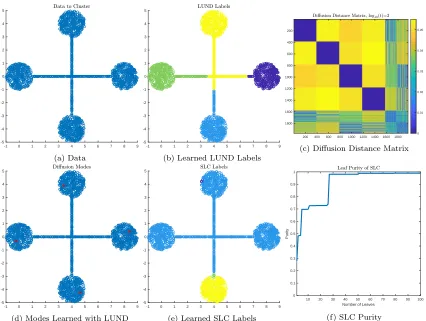
LUND is related to SLC in the sense that the underlying density of the data is an important determinant in the clusterings. However, LUND also incorporates geomet-ric structure in the data when determining clusters, which can be especially powerful when density is uninformative. In Figure 4, data with constant density but significant geometric structure is analyzed. LUND succeeds in learning an accurate clustering with respect to the latent data geometry, while SLC fails. A theoretical analysis of the bottleneck phenomenon is presented in Section 4.3.
4. Analysis of Diffusion Processes on Data
In this section, we derive estimates for diffusion distances. LetDin
t , Dbtwt be as in (3.2).
The main result of this section is to show there exists a time intervalT ⊂[0,∞] so that
∀t∈ T, Dtbtw> Dtin,that is, fort∈ T, within cluster diffusion distance is smaller than
between cluster diffusion distance. Showing that within-cluster distances are small and between-cluster distances are large is essential for any clustering problem. The benefit of using diffusion distance is its adaptability to the geometry of the data: it is possible that within cluster diffusion distance is less than between cluster diffusion distance, even in the case that the clusters are highly elongated and nonlinear. This property does not hold when points are compared with Euclidean distances or many other data-independent distances.
-1 0 1 2 3 4 5 6 7 8 9 -5 -4 -3 -2 -1 0 1 2 3 4 5 (a) Data
-1 0 1 2 3 4 5 6 7 8 9 -5 -4 -3 -2 -1 0 1 2 3 4 5
(b) Learned LUND Labels
200 400 600 800 1000 1200 1400 1600 1800 200 400 600 800 1000 1200 1400 1600 1800 0 0.01 0.02 0.03 0.04 0.05
(c) Diffusion Distance Matrix
-1 0 1 2 3 4 5 6 7 8 9 -5 -4 -3 -2 -1 0 1 2 3 4 5
(d) Modes Learned with LUND
-1 0 1 2 3 4 5 6 7 8 9 -5 -4 -3 -2 -1 0 1 2 3 4 5
(e) Learned SLC Labels
10 20 30 40 50 60 70 80 90 100 Number of Leaves
0 0.1 0.2 0.3 0.4 0.5 0.6 0.7 0.8 0.9 1 Purity
(f) SLC Purity
Figure 4: Geometric data with roughly constant empirical density is shown in (a). The spherical clusters are connected with thin bottlenecks. In (d), the modes learned by LUND are shown in red, indicating that one mode per cluster is learned. This is because although the density is roughly constant, the thin bottlenecks force the four circular clusters to be far apart in diffusion distance. The corresponding labels learned by LUND are in (b), showing that the cluster structure is accurately inferred. In (c), the matrix of pairwise diffusion distances is shown with diffusion time t= 103 and
diffusion scaling parameterσ=.5. The four blue blocks on the diagonal indicate that within-cluster diffusion distances are small, while between cluster diffusion distances are large. The connecting bottlenecks correspond to the final rows and columns of this matrix, where the diffusion distances are less informative. In (e), labels learned from pruning the single linkage dendrogram at the third highest merge (producing four clusters) is shown, indicating this method is not appropriate for this data. Indeed, in (f), the purity of the hierarchical clustering is shown as a function of how many leaves (i.e. clusters) are used from the dendrogram. The purity remains low until ∼ 25 clusters are used, indicating that the single linkage dendrogram is unable to efficiently separate the four spherical clusters until ∼25 clusters are used. The fundamental reason for the failure of SLC on this data is the fact that the density is essentially constant and the data set is connected, which are the properties driving SLC. Unlike LUND, SLC does not incorporate geometric information, e.g. bottlenecks, which is quite discriminative for this data set.
4.1 Near Reducibility of Diffusion Processes
For any initial distribution π0, limt→∞π0Pt = π and moreover for any choice of
ν = π0/π, Dt(x, y) → 0 uniformly as t → ∞. One can quantify the rate of this
convergence by estimating the convergence rate of Pto its stationary distribution. Definition 4.1 For a discrete Markov chain with transition matrixPand stationary
distributionπ, the relative pointwise distance toπ at timet is∆(t) = max
i,j∈{1,...,n}|P
t
ij−
πj|/πj.
The decay of ∆(t) is regulated by the spectrum of P (Jerrum and Sinclair, 1989; Sinclair and Jerrum, 1989). Indeed, let 1 = λ1 > λ2 ≥ · · · ≥ λn > −1 be the
eigenvalues of P; note that λ2 < 1 follows from P irreducible and λn > −1 follows
from Paperiodic (Chung, 1997). Let λ∗ = maxi=2,...,n|λi|= max(|λ2|,|λn|), πmin = minx∈Xπ(x).
Theorem 4.2 (Jerrum and Sinclair, 1989; Sinclair and Jerrum, 1989) Let Pbe the
transition matrix of a Markov chain on state spaceX satisfying the usual assumptions.
Then ∆(t)≤λt∗/πmin.
Instead of analyzing λ∗, the conductance of X may be used to bound ∆(t).
Definition 4.3 Let G be a weighted graph on X and let S ⊂ X. The conductance of S is ΦX(S) = P
xi∈S,xj∈Sc
πiPij/min Pxi∈Sπi,
P
xi∈Scπi
. The conductance of G
is Φ(P) = minS⊆GΦX(S).
Methods for estimating the conductance of certain graphs includePoincar´e estimates
(Diaconis and Stroock, 1991; Diaconis and Saloff-Coste, 1993) and the method of
canonical paths (Jerrum and Sinclair, 1989; Sinclair and Jerrum, 1989; Aldous and
Fill, 2002). These approaches estimate Φ(P) by showing that certain simple paths may be used as surrogates for generic paths in the graph. The conductance is related toλ2; see Chung (1997):
Theorem 4.4 (Cheeger’s Inequality) LetGbe a weighted, undirected graph with
tran-sition matrix P. Then the second eigenvalue λ2 of P satisfies Φ(P)2/2 ≤ 1−λ2 ≤
2Φ(P).
Combining Theorem 4.2 and Cheeger’s inequality relates ∆(t) to Φ(P).
Theorem 4.5 (Jerrum and Sinclair, 1989; Sinclair and Jerrum, 1989) Let Pbe the
transition matrix for a Markov chain onX satisfying the usual assumptions. Suppose
Note that any Markov chain can be made to satisfy Pii ≥ 12,∀i= 1, . . . , n, simply by
replacing P with 1
2(P+I). This keeps the same stationary distribution and reduces the conductance by a factor of 12.
Whether Theorem 4.2 or 4.5 is used, the convergence of P towards its stationary distribution is exponential, with rate determined byλ∗ or Φ(P), that is, to how close to being reducible the chain is. This yields estimates on diffusion distances; indeed, for x, y ∈X and any initial distributionπ0,
Dt(x, y) =||pt(x,·)−pt(y,·)||`2(ν) ≤ ||pt(x,·)−π(·)||`2(ν)+||pt(y,·)−π(·)||`2(ν)
≤2
s X
u∈X
max
z∈X
|pt(z, u)−π(u)|2
π(u)2 π(u)π0(u)
≤2∆(t)
s X
u∈X
π(u)π0(u)≤2∆(t)≤
2(1− 1 2Φ(P)
2)t
πmin
.
Thus, as t → ∞, Dt → 0 uniformly at an exponential rate depending on the
con-ductance of the underlying graph; a similar result holds for λ∗ in place of Φ(P). This gives a global estimate on the diffusion distance in terms of λ∗ and Φ(P). Note that a similar conclusion holds by analyzing (2.2), recalling that ψ1 is constant and
λ2 = maxi6=1|λi|=λ∗.
Unfortunately, a global estimate on diffusion distances may be too coarse for unsuper-vised clustering. To obtain the desired separation ofDint , Dtbtw, we need to study not the global mixing time, but the mesoscopic mixing times, corresponding to the time it takes for convergence of points in each cluster towards their mesoscopic equilibria, before reaching the global equilibrium. For this purpose, we use results from the theory of nearly reducible Markov processes (Simon and Ando, 1961; Meyer, 1989). Suppose the matrix P is irreducible; write P, possibly after a permutation of the indices of the points, in block decomposition as
P=
P11 P12 . . . P1m
P21 P22 . . . P2m
..
. ... . .. ...
Pm1 Pm2 . . . Pmm
, (4.6)
where eachPii is square andm≤n. LetIi be the indices of the points corresponding
to Pii. Recall that if the graph corresponding to P is disconnected, then P is a
reducible Markov chain. Recall that kAk∞= maxiPj|Aij| is the maximal row sum
of A = (Aij). Suppose that kPijk∞ is small but nonzero for i 6= j, that is, most of the interactions for points in Ii are contained within Pii. This suggests diffusion
on the blocks Pii have dynamics that converge to their own, mesoscopic equilibria
before the entire chain converges to a global equilibrium, depending on the weakness of connection between blocks. Interpreting the support sets Ii as corresponding to
each cluster are close in diffusion distance but far in diffusion distance from points in other clusters; such a state corresponds to a mesoscopic equilibrium. To make this precise, consider the notion of stochastic complement.
Definition 4.7 Let Pbe an n×n irreducible Markov matrix partitioned into square
block matrices as in (4.6). For a given indexi∈ {1, . . . , m}, letPi denote the principal
block submatrix generated by deleting the ith row and ith column of blocks from (4.6),
and letP∗i =
P1iP2i. . .Pi−1,iPi+1,i. . .Pmi
T
andPi∗ =
Pi1 Pi2 . . . Pi,i−1 Pi,i+1 . . . Pim
. The stochastic complement of Pii is the matrix Sii =Pii+Pi∗(I−Pi)−1P∗i.
One can interpret the stochastic complementSiias the transition matrix for a reduced
Markov chain obtained from the original chain, but in which transitions into or out ofIi are masked. More precisely, in the reduced chainSii, a transition is either direct
inPii or indirect by moving first through points outside ofPii, then back into Pii at
some future time. Indeed, the termPi∗(I−Pi)−1P∗i in the definition ofSii accounts
for leaving Ii (the factor Pi∗), traveling for some time in Iic (the factor (I−Pi)−1),
then re-enteringIi (the factorP∗i). Note that the factor (I−Pi)−1 may be expanded
in Neumann sum as (I−Pi)−1 =
P∞
t=0P
t
i, showing that it accounts for exiting from Ii and returning to it after an arbitrary number of steps outside of it.
The notion of stochastic complement quantifies the interplay between the mesoscopic and global equilibria of P. We say P is primitive if it is non-negative, irreducible and aperiodic. The following theorem indicates how P may be analyzed when it is derived from cluster data {Xk}Kk=1 sampled according to (3.1); a proof appears in the Appendix for completeness. This result, which produces estimates related to the diffusion operator P in the `1 norm, is used to prove results on diffusion distances, which are defined in an `2 sense, partially in order to take advantage of spectral decompositions for fast computations. This discrepancy will be discussed and controlled in Section 4.2.
Theorem 4.8 (Meyer, 1989) Let P be an n ×n irreducible row-stochastic matrix
partitioned into K2 square block matrices, and let S be the reducible row-stochastic
matrix consisting of the stochastic complements of the diagonal blocks of P:
P=
P11 P12 . . . P1K
P21 P22 . . . P2K
..
. ... . .. ...
PK1 PK2 . . . PKK
, S=
S11 0 . . . 0
0 S22 . . . 0
..
. ... . .. ...
0 0 . . . SKK
.
Suppose each Sii is primitive, so that the eigenvalues of S satisfy λ1 = λ2 = · · · =
λK = 1> λK+1 ≥λK+2 ≥ · · ·>−1. Let Z diagonalize S, and let
S∞= lim
t→∞S
t=
1π1 0 . . . 0
0 1π2 . . . 0
..
. ... . .. ...
0 0 . . . 1πK
where πi is the stationary distribution for Sii. Then kPt−S∞k∞ ≤ tδ +κ|λK+1|t,
where δ = 2 maxikPi∗k∞ and κ =kZk∞kZ−1k∞. Moreover, for any initial
distribu-tion π0 and s= limt→∞π0St =π0S∞, kπ0Pt−sk1 ≤tδ+κ|λK+1|t.
Note that this result does not require the Markov chain to be reversible, and hence applies to diffusion processes defined on directed graphs. The assumption that S is diagonalizable is not strictly necessary, and similar estimates hold more generally (Meyer, 1989).
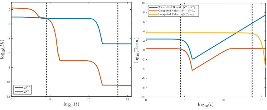
The estimatetδ+κ|λK+1|t consists of two terms. Thetδ term corresponds tokPt− Stk∞, which accounts for the approximation of Pt by the reducible Markov chain St. In the context of clustering, this term accounts for the between-cluster connections in P. The term κ|λK+1|t corresponds to kSt−S∞k∞, which accounts for propensity of mixing within a cluster. In the clustering context, this term quantifies the within-cluster distances.
It follows from Theorem 4.8 that, given sufficiently large, there is a range of t
for which the dynamics of Pt are -close to the dynamics of the reducible, low-rank Markov chain S∞.
Corollary 4.9 Let λK+1, δ, κ be as in Theorem 4.8. Suppose that for some >0, ln 2κ
/ln|λ1
K+1|
< t < 2δ. Then kPt−S∞k
∞< , and for every initial distribution
π0, kπ0Pt−sk1 < .
In contrast with t, the values λK+1, δ, κ may be understood as fixed geometric pa-rameters of the data set which determine the range of times t at which mesoscopic equilibria are reached. More precisely, asn → ∞,δ, κconverge to natural continuous quantities independent of n, and Garcia Trillos et al. (2018) proved that as n → ∞, there is a natural scaling forσ →0+ in which the (random) empirical eigenvalues of P converge in a precise sense to the (deterministic) eigenvalues of a corresponding continuous operator defined on the support of µ as in (3.1). Thus, the parameters of Theorem 4.9 may be understood as random fluctuations of geometrically intrin-sic quantities depending on µ. In the context of the proposed data model, these quantities may be interpreted as follows:
• λK+1 is the largest eigenvalue ofS not equal to 1. SinceSis block diagonal and each Skk is primitive, it follows that λK+1 = maxk=1,...,Kλ2(Skk). As discussed
above, {λ2(Skk)}Kk=1 is related to the conductance Φ(Skk) and the mixing time
of the random walk restricted to Skk. If the entries ofSkk are very close to the
entries of Pkk, then a perturbative argument yields λ2(Skk)≈λ2(Pkk).
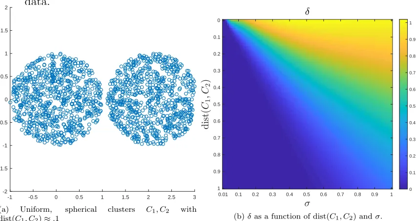
n sufficiently large, dist(C1, C2) = minx1∈C1,x2∈C2kx1−x2k2 ≈η. Note that the
point in B1(0,0) nearest B1(2 +η,0) is (1,0). Then modulo the variance from the random sampling,
δ≈
2
Z
B1(2+η,0)
exp(−k(x, y)−(1,0)k2 2/σ
2)dxdy
Z
B1(2+η,0)
exp(−k(x, y)−(1,0)k2 2/σ
2)dxdy+
Z
B1(0,0)
exp(−k(x, y)−(1,0)k2 2/σ
2)dxdy
≤ 2 exp(−η
2/σ2) exp(−(η2+ 4η)/σ2) + 1.
(4.10)
Figure 5 illustrates empirically how δ depends on σ and dist(C1, C2) for such data.
-1 -0.5 0 0.5 1 1.5 2 2.5 3 -2
-1.5 -1 -0.5 0 0.5 1 1.5 2
(a) Uniform, spherical clusters C1, C2 with
dist(C1, C2)≈.1
0.01 0.1 0.2 0.3 0.4 0.5 0.6 0.7 0.8 0.9 1 0
0.1
0.2
0.3
0.4
0.5
0.6
0.7
0.8
0.9
1 0
0.1 0.2 0.3 0.4 0.5 0.6 0.7 0.8 0.9 1
(b)δas a function of dist(C1, C2) andσ.
Figure 5: In (a), data drawn uniformly at random from the union of two balls inR2is shown. In (b),
it is shown that for such equal sized, spherical, constant density clusters, the separation parameter exhibits rapid decay asσ→0+, for fixed separation. The experiments confirm that the decay of δ
is essentially logistic in−(η2/σ2), as estimated in (4.10).
• The quantity κ = kZk∞kZ−1k∞, with Z = (φ1|. . .|φn), is a measure of the
4.2 Diffusion Distance Estimates
Returning to the proposed data model X = SK
k=1Xk ∼ µ as per (3.1), let P be a
corresponding Markov chain on X satisfying the usual assumptions. We estimate the dependence of diffusion distances on the parameters δ, λK+1, κ above. We also intro-duce abalance quantity that quantifies the difference between the`1 norm (the setting of Theorem 4.8) and the`2 norm (the setting of diffusion distances). Throughout this section, let pt(xi, xj) = Ptij, s
∞(x
i, xj) =S∞ij.
Definition 4.11 Let P,S∞∈Rn×n be as in Theorem 4.8. Define
γ(t) = max
x∈X 1−
1 2
X
u∈X
|pt(x, u)−s∞(x, u)|
kpt(x,·)−s∞(x,·)k2
− √1
n
2!−1
.
Botelho-Andrade et al. (2019) show that for any vectorv ∈Rn,kvk
2 = √cvnkvk1,where
cv = 1−
1 2
n
X
i=1
|vi|
kvk2
− √1
n
2!−1
.
In this sense, γ(t) measures how the `1 norm differs from the `2 norm across all rows of Pt−S∞. In particular, when each row of Pt−S∞ is close to uniform,γ(t) is close to 1; when some row of Pt−S∞ concentrates all its mass around one index, then
γ(t) = √n. Note that 1≤γ(t)≤√n for all t.
Theorem 4.12 Let X = SK
k=1Xk and let P be a corresponding Markov transition
matrix onX. Letδ, λK+1, κ,S∞ be as in Theorem 4.8. LetDtbe the diffusion distance
associated to P and counting measure ν. If t, satisfy
ln 2κ lnλ 1
K+1
< t <
2δ,
then
(a) Dint ≤2√
nγ(t).
(b) Dbtwt ≥2 min
y∈X ks
∞
(y,·)k`2(ν)−2
√
nγ(t).
ProofBy Corollary 4.9,kPt−S∞k
∞< , that is, maxx∈X
P
u∈X |pt(x, u)−s∞(x, u)|ν(u)<
. To see (a), let k be arbitrary and let x, y ∈Xk. Then:
||pt(x,·)−pt(y,·)||`2(ν)
=√1
n 1−
1 2
X
u∈X
|pt(x, u)−s∞(x, u)|
kpt(x,·)−s∞(x,·)k`2(ν)
− √1
n
2!−1
||pt(x,·)−s∞(x,·)||`1(ν)
+√1
n 1−
1 2
X
u∈X
|pt(y, u)−s∞(y, u)|
kpt(y,·)−s∞(y,·)k`2(ν)
− √1
n
2!−1
||pt(y,·)−s∞(y,·)||`1(ν)
+||s∞(y,·)−s∞(x,·)||`2(ν)
≤√2
nmaxx∈X 1−
1 2
X
u∈X
|pt(x, u)−s∞(x, u)|
kpt(x,·)−s∞(x,·)k`2(ν)
− √1
n
2!−1
+||s∞(y,·)−s∞(x,·)||`2(ν),
where t satisfies ln 2κ/lnλ 1 K+1
< t < /(2δ). The line relating the norm in
`1(ν) and `2(ν) follows from Theorem 1 in Botelho-Andrade et al. (2019). Note that S∞ has constant columns on each cluster, and in particular for x, y ∈ Xk,
s∞(x, u) = s∞(y, u) = πk(u) for all u ∈ X, so that ||s∞(y,·)−s∞(x,·)||`2(ν) = 0.
Statement (a) follows.
To see (b), suppose thatx∈Xk, y ∈X`, k 6=`. Then
kpt(x,·)−pt(y,·)k`2(ν)
=kpt(x,·)−s∞(x,·) +s∞(x,·)−s∞(y,·) +s∞(y,·)−pt(y,·)k`2(ν)
≥ks∞(x,·)−s∞(y,·)k`2(ν)− kpt(x,·)−s∞(x,·)k`2(ν)− kpt(y,·)−s∞(y,·)k`2(ν)
=ks∞(x,·)−s∞(y,·)k`2(ν)
−√1
n 1−
1 2
X
u∈X
|pt(x, u)−s∞(x, u)|
kpt(x,·)−s∞(x,·)k`2(ν)
− √1
n
2!−1
||pt(x,·)−s∞(x,·)||`1(ν)
−√1
n 1−
1 2
X
u∈X
|pt(y, u)−s∞(y, u)|
kpt(y,·)−s∞(y,·)k`2(ν)
− √1
n
2!−1
||pt(y,·)−s∞(y,·)||`1(ν)
≥ks∞(x,·)−s∞(y,·)k`2(ν)−
√
n 1−
1 2
X
u∈X
|pt(x, u)−s∞(x, u)|
kpt(x,·)−s∞(x,·)k`2(ν)
− √1
n
2!−1
−√
n 1−
1 2
X
u∈X
|pt(y, u)−s∞(y, u)|
kpt(y,·)−s∞(y,·)k`2(ν)
− √1
n
2!−1
≥ks∞(x,·)−s∞(y,·)k`2(ν)−2
√
n z∈maxX`∪Xk
1− 1
2
X
u∈X
|pt(z, u)−s∞(z, u)|
kpt(z,·)−s∞(z,·)k`2(ν)
− √1
n
2!−1
≥2 min
w∈Xk∪X`
ks∞(w,·)k`2(ν)−2
√
nz∈maxX`∪Xk
1− 1
2
X
u∈X
|pt(z, u)−s∞(z, u)|
kpt(z,·)−s∞(z,·)k`2(ν)
−√1
n
2!−1
,
where in the last step, to lower bound the first term we used that s∞(y,·) = πl(·),
are disjoint. Minimizing this lower bound over all clusters Xk, X` yields the desired
result.
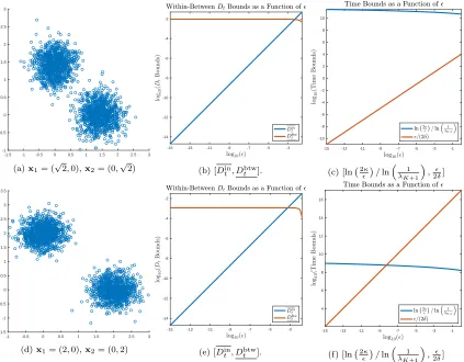
Heuristically, if is small and the reduced equilibrium distribution s∞ is roughly constant on each cluster, there will be a range oft for whichDin
t Dtbtw.The notion
of s∞ being roughly constant on each cluster is equivalent to nodes in the same cluster having roughly constant degree. These theoretical estimates are compared to empirical bounds computed numerically in Section 6.
If P is very close to S in Frobenius norm, then pt(x, y) is very close to s∞(x, y) and may be taken close to 0. In particular, for the ideal case = 0, the estimates of Theorem 4.12 reduce to
Dtin= 0 , Dtbtw≥2 min
y∈Xks
∞
(y,·)k`2(ν). (4.13)
One can define a natural notion of diffusion distance between disjoint clusters in a reducible Markov chain as the sum of the `2 norms of their respective stationary distribution, which agrees with both the definition of diffusion distances upon taking the limit t → +∞ and with the lower bound (b) in Theorem 4.12 when → 0+. Hence, while the estimates in the proof of Theorem 4.12 may not be optimal, they are quite natural for →0+.
Away from the asymptotic regime → 0+, the estimates of Theorem 4.12 may be further simplified by placing additional assumptions on the data. Indeed, if the equilibrium distributions inS∞ are balanced and uniform, the following result holds: Corollary 4.14 Suppose that s∞ is uniform on each Xk, and the cardinality of each
Xk isn/K. Then for any t, satisfying ln 2κ
ln 1
λK+1
< t <
2δ,
Dtin ≤ √2
nγ(t) , D
btw
t ≥
2
√
n
√
K −γ(t)
.
Proof If S∞ has constant rows on each cluster (i.e. the stationary distribution on each cluster of the reduced Markov chain is uniform), and the clusters are of constant size n/K, then 2 miny∈Xks∞(y,·)k`2(ν) = 2
p
K/n. Then Theorem 4.12 yields
Dbtwt ≥2 min
y∈X ks
∞
(y,·)k`2(ν)−2
√
nγ(t)
=2
r
K
n −2
√
nγ(t)
=√2
n
√