Dependent relevance determination for smooth and
structured sparse regression
Anqi Wu [email protected]
Princeton Neuroscience Institute Princeton University
Princeton, NJ 08544, USA
Oluwasanmi Koyejo [email protected]
Beckman Institute for Advanced Science and Technology Department of Computer Science
University of Illinois at Urbana-Champaign Urbana, Illinois, 61801, USA
Jonathan Pillow [email protected]
Princeton Neuroscience Institute Princeton University
Princeton, NJ 08544, USA
Editor:David Wipf
Abstract
In many problem settings, parameter vectors are not merely sparse but dependent in such a way that non-zero coefficients tend to cluster together. We refer to this form of dependency as “region sparsity.” Classical sparse regression methods, such as the lasso and automatic relevance determination (ARD), which model parameters as independent a priori, and therefore do not exploit such dependencies. Here we introduce a hierarchical model for smooth, region-sparse weight vectors and tensors in a linear regression setting. Our ap-proach represents a hierarchical extension of the relevance determination framework, where we add a transformed Gaussian process to model the dependencies between the prior vari-ances of regression weights. We combine this with a structured model of the prior varivari-ances of Fourier coefficients, which eliminates unnecessary high frequencies. The resulting prior encourages weights to be region-sparse in two different bases simultaneously. We develop Laplace approximation and Monte Carlo Markov Chain (MCMC) sampling to provide effi-cient inference for the posterior. Furthermore, a two-stage convex relaxation of the Laplace approximation approach is also provided to relax the inevitable non-convexity during the optimization. We finally show substantial improvements over comparable methods for both simulated and real datasets from brain imaging.
Keywords: Bayesian nonparametric, Sparsity, Structure learning, Gaussian Process, fMRI
c
1. Introduction
Recent work in statistics has focused on high-dimensional inference problems in which the number of parameters equals or exceeds the number of samples. We focus specifically on
the linear regression setting: consider a scalar response yi ∈ R generated from an input
vectorxi ∈Rp via the linear model:
yi =xi>w+i, for i= 1,2,· · ·, n, (1)
with observation noise i ∼ N(0, σ2). The regression (linear weight) vector w ∈ Rp is
the quantity of interest. This general problem is ill-posed when n ≤ p. However, it is
surprisingly tractable when w has special structure, such as sparsity in an appropriate
basis. A large literature has provided theoretical guarantees about the solvability of such problems, as well as a suite of practical methods for solving them.
Methods based on simple sparsity such as the lasso (Tibshirani, 1996) typically treat
regres-sion weights as independent a priori. This neglects a statistical feature of many real-world
problems, which is that non-zero weights tend to arise in local groups or clusters. In many problem settings, weights have an explicit geometric relationship, such as indexing in time (e.g., time series regression) or space (e.g., brain imaging data). If a single regression weight is non-zero, nearby weights in time or space are also likely to be non-zero. Conversely, in a region where most weights are zero, any particular coefficient is also likely to be zero. Thus, nearby weights exhibit dependencies that are not captured by independent priors. We refer
to this form of dependency asregion sparsity.
A variety of methods have been developed to incorporate local dependencies between re-gression weights, such as the group lasso (Yuan and Lin, 2006). However, these methods typically require the user to pre-specify the group size or to partition the weights into groups a priori. Such information is unavailable in many applications of interest, and hard par-titioning into groups breaks dependencies between nearby coefficients that are assigned to different groups.
In this paper, we take a Bayesian approach to inferring regression weights with region-sparse
structure. We introduce a hierarchical prior overwof the form:
u∼ GP (2)
w|u∼ N(0, C(u)), (3)
where u is a latent vector that captures dependencies in the sparsity pattern of w, and
w|u has a zero-mean Gaussian distribution with a diagonal covariance matrix C(u), given
by a deterministic function of u. We use a Gaussian process (GP) prior over u to encode
structural assumptions about region sparsity (e.g., the typical size of clusters of non-zero weights and the spacing between them). This model can be seen as an extension of
auto-matic relevance determination (ARD), in which the elements ofu area prioriindependent
(MacKay, 1992; Neal, 1995). We therefore refer to it as dependent relevance determination
(DRD).
This is reflected in the fact that we define the DRD prior covariance matrix C(u) to be
diagonal, making the weights conditionally independent given the pattern defined byu. In
many cases, however, we expect weights to be smooth as well as sparse due to the conti-nuity of the input regressors in space or time. Most of the real datasets do exhibit spatial and temporal correlations. Coefficients usually possess contiguous regions and smoothness. Hence, we are aiming at developing a universal approach easily integrating both structured sparsity and smoothness concurrently. To incorporate smoothness, we combine the stan-dard DRD prior with a squared exponential covariance function. The resulting prior has a non-diagonal covariance matrix that encourages smoothness as well as sparsity. We refer to
this extension as smooth dependent relevance determination(smooth-DRD). Samples from
the smooth-DRD prior have local islands of smooth and non-zero weights, surrounded by large regions of zeros. We will show that combining region-sparsity and smoothness together will significantly enhance the performance in a non-trivial way.
Unfortunately, exact inference under DRD and smooth-DRD priors is analytically intractable. We therefore introduce an approximate inference method based on a Laplace approximation
to the posterior overu, and a sampling-based inference method using Monte Carlo Markov
Chain (MCMC) sampling. We also derive a two-stage convex relaxation of the Laplace approximation approach in order to overcome the effects of bad local optima.
We show experimental evaluations on 1D simulated datasets comparing the performance among different methods. In addition, the phase transition curve analyses are carried out against lasso to show the superiority of DRD and smooth-DRD in support recovery for group structure sparsity with or without smoothness. Furthermore, the DRD based pri-ors are exploited for three brain imaging datasets. Domain expertise and current evidence in brain imaging suggest that discrimination performance is primarily driven by spatially smooth activation within spatially sparse regions, and several estimation algorithms have been proposed that exploit this structure (Grosenick et al., 2011; Michel et al., 2011; Bal-dassarre et al., 2012; Gramfort et al., 2013). We provide experimental comparisons to these methods, showing the superiority of DRD in practice. In particular, DRD provides spa-tial decoding weights for brain imaging data that are both more interpretable and achieve higher decoding performance.
Here we highlight our key contributions as follows:
• We introduce a new hierarchical model for smooth, region-sparse weight tensors. The
model uses a Gaussian process to introduce dependencies between prior variances of regression weights governing localized sparsity in weights and simultaneously imposes smoothness by integrating a smoothness-inducing covariance function into the prior distribution of weights.
• We describe two methods for inferring the model parameters: one based on the Laplace
• We show phase transition curves governing the transition from imperfect to near-perfect recovery for lasso and DRD estimators, revealing that group structure and smoothness can have a major impact on the recoverability of sparse signals.
This paper is organized as follows. In Sec. 2, we review the related structured sparsity literature. In Sec. 3, we introduce our new region-sparsity and smoothness inducing priors. In Sec. 4, we propose two approaches to Bayesian inference for parameter estimation, the evidence optimization via Laplace approximation and the MCMC sampling. A two-stage convex relaxation of the Laplace approximation approach is also introduced to alleviate the non-convexity with a more robust two-stage convexity. Sec. 5 introduces a detailed analysis of the structured sparsity and smoothness properties of the DRD based priors and the other methods that can be used for this purpose. Sec. 6 presents the phase transition analysis for lasso and DRD estimators. Sec. 7 shows some experiments on three real brain imaging datasets, comparing different methods that can be used for structured sparsity. Finally, Sec. 8 presents the conclusion and discussion of this work.
2. Related work
The classic method for sparse variable selection is the lasso, introduced by Tibshirani (1996),
which places anl1 penalty on the regression weights. This method can be interpreted as a
maximum a posteriori (MAP) estimate under a Laplace (or double-exponential) prior. A fully Bayesian treatment of this model was later developed by Park and Casella (2008). A variety of Bayesian methods based on other sparsity-inducing prior distributions have been developed, including the horseshoe prior (Carvalho et al., 2009), which uses a continuous density with an infinitely tall spike at the origin and heavy tails, and the spike-and-slab prior (Mitchell and Beauchamp, 1988) which consists of a weighted mixture of a delta function (the spike) and a broad Gaussian (the slab), both centered at the origin.
Another approach to sparse variable selection comes from empirical Bayes (also known as evidence optimization or “type-II” marginal likelihood). These methods rely on a two-step inference procedure: (1) optimize hyperparameters governing the sparsity pattern via ascent of the marginal likelihood; and then (2) compute MAP estimates of the parameters given the hyperparameters. The most popular such estimator is automatic relevance determination (ARD), which prunes unnecessary coefficients by optimizing the precision of each regression
coefficient under a Gaussian model (MacKay, 1992; Neal, 1995). The relevance vector
machine (RVM) was later formulated as a general Bayesian framework for obtaining sparse solutions to regression and classification tasks (Tipping, 2001). The RVM has an identical functional form to the support vector machine, but provides probabilistic analysis. Tipping and Faul (2003) then was proposed for RVM to scale up its training procedure.
All these methods can be interpreted as imposing a sparse and independent prior on the regression weights. The resulting posterior over weights has high concentration near the axes, so that many weights end up at zero unless forced away strongly by the likelihood.
They achieved the group sparse structure by introducing an l1 penalty on thel2 norms of
each group. Moreover, Huang et al. (2011) generalized the group sparsity idea by using coding complexity regularization methods associated with the structure. A variety of other papers have proposed alternative approaches to correlated or structured regularization (Ja-cob et al., 2009; Liu et al., 2009; Kim and Xing, 2009; Friedman et al., 2010; Jenatton et al., 2011; Kowalski et al., 2013).
Previous literature has also explored Bayesian methods for structured sparse inference. A common strategy is to introduce a latent multivariate Gaussian that controls the correla-tion structure governing condicorrela-tionally independent densities over coefficients. Gerven et al. (2009) extended the univariate Laplace prior to a novel multivariate Laplace distribution
represented as a scale mixture that induces coupling. Hern´andez-Lobato and Hern´
andez-Lobato (2013) described a similar approach that results in a marginally horseshoe prior. Several other papers have proposed dependent generalizations of the spike-and-slab prior.
Hern´andez-Lobato et al. (2013) described a group spike-and-slab distribution using a
mul-tivariate Bernoulli distribution over the indicators of the spikes associated with a group specification. Subsequently, Andersen et al. (2014, 2015) relaxed the hard-coded group specification by encoding the structure with a generic covariance function. Meanwhile, En-gelhardt and Adams (2014) introduced a Bayesian model for structured sparsity that uses a Gaussian process (GP) to control the mixing weights of the spike and slab prior in propor-tion to feature similarity. Apart from imposing the correlapropor-tion structure on the independent spike and slab elements, Yu et al. (2012) put forward a hierarchical Bayesian framework with the mixing weights of the cluster patterns generated from Beta distributions. Our work is most similar to Engelhardt and Adams (2014) and Andersen et al. (2015), except that we use an ARD-like approach with a conditionally Gaussian density over coefficients instead of a spike and slab prior. Our work is also the first that we are aware of that simultaneously captures sparsity and smoothness.
3. Dependent relevance determination (DRD) priors
In this section, we introduce the DRD prior and the smooth-DRD prior, an extension to incorporate smoothness of regression weights. We focus on the linear regression setting with conditional responses distributed as:
y|X,w, σ2 ∼ N(y|Xw, σ2I), (4) where X = [x1, . . . ,xn]> ∈Rn×p denotes the design matrix,y = [y1,· · ·, yn]> ∈Rn is the
observation vector, and σ2 is the observation noise variance, where p is the dimension of
the input vectors andn is the number of samples.
3.1. Automatic relevance determination
The relevance determination framework includes a family of estimators that rely on a zero-mean multivariate normal prior:
hyper-parameters
weights
likelihood
sparsity
latent variables
weights
likelihood
ARD
DRD
smooth-DRD
sparsity
smoothness latent
variables
weights
likelihood
A
B
C
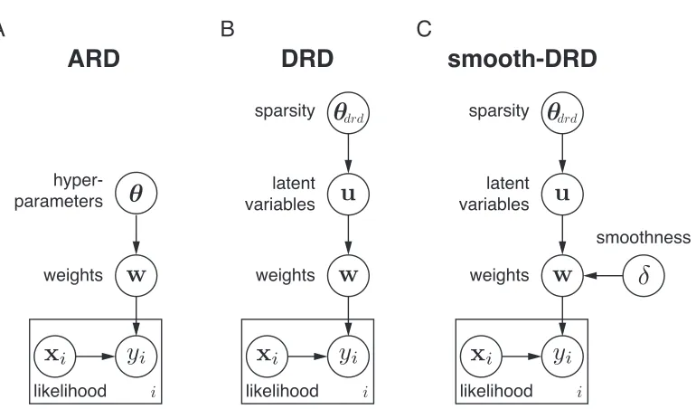
Figure 1: Graphical models for ARD, DRD and smooth-DRD.
where the prior covariance matrixC(θ) is a function of some hyperparametersθ. The form
of the dependence ofConθleads to different forms of assumed structure, including sparsity
(Tipping, 2001; Faul and Tipping, 2002; Wipf and Nagarajan, 2008), smoothness (Sahani and Linden, 2003; Schmolck, 2008), or locality (Park and Pillow, 2011).
Automatic relevance determination (ARD) defines the prior covariance to be diagonal,Cii=
θ−i 1, where a distinct hyperparameter θi specifies the prior precision for the i’th regression
coefficient. ARD places an independent improper gamma prior on each hyperparameter,
θi ∼gamma(0,0), and performs inference for {θi} by maximizing the marginal likelihood.
This sends many θi to infinity, pruning the corresponding coefficients out of the model. A
typical graphical model for ARD is presented in Fig. 1A. The independence assumption in the prior over hyperparameters means that there is no tendency for nearby coefficients to remain in or be pruned from the model. This is the primary shortcoming that our method seeks to overcome.
3.2. DRD: A hierarchical extension of ARD
We extend the standard ARD model by adding a level of hierarchy. Instead of directly optimizing hyperparameters that control sparsity of each weight, as in ARD, we introduce a latent vector governed by a GP prior to capture dependencies in the sparsity pattern over
weights (see Fig. 1B). Letu∈Rp denote a latent vector distributed according to a GP prior
where b∈R is the scalar mean, 1 is a length-p vector of ones, and covariance matrix K is
determined by a squared exponential kernel. Thei, j’th entry of K is given by
Kij =ρexp
−||χi−χj||
2
2l2
, (7)
where χi and χj are the spatial locations of weights wi and wj, respectively, and kernel
hyperparameters are the marginal varianceρ >0 and length scalel >0. Samples from this
GP on a grid of locations{χi}are smooth on the scale ofl, and have meanb and marginal
varianceρ.
To obtain a prior over region-sparse weight vectors, we transform u to the positive values
via a nonlinear function f, and the transformed latent vector g =f(u) forms the diagonal
of a diagonal covariance matrix for a zero-mean Gaussian prior over the weights:
Cdrd= diag
h f(u)
i
, (8)
where f is a monotonically increasing function that squashes negative values of u to near
zero. Here we will mainly consider the exponential functionf(u) = exp(u), but we will also consider “soft-rectification” functionf(u) = log(1 + exp(u)) in the experiment for numerical
stability. When the GP mean b is very negative relative to the prior standard deviation
√
ρ, most elements of g will be close to zero, resulting in weights w with a high degree of
sparsity (i.e., few weights far from zero). The length scale l determines the smoothness of
samplesu and thereby determines the typical width of bumps in the prior varianceg. We
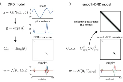
denote the set of hyperparameters governing the GP prior onu byθdrd ={b, ρ, l}. Fig. 2A
shows a depiction of sampling from the DRD generative model.
3.3. Smooth-DRD
The standard DRD model imposes smooth dependencies in the prior variances of the regres-sion weights, but the weights themselves remain uncorrelated (as reflected by the fact that
the covariance Cdrd is diagonal). In many settings, however, we expect weights to exhibit
smoothness in addition to region sparsity. To capture this property, we can augment DRD with a second Gaussian process, denoted as smooth-DRD, that induces smoothness, con-tributing off-diagonal structure to the prior covariance matrix while preserving the marginal variance pattern imposed by DRD (see Fig. 1C).
Let Σ denote a covariance matrix governed by a standard squared-exponential GP kernel:
Σij = exp
−||χi−χj||
2
2δ2
, (9)
with length scaleδand marginal variance set to 1. Then we define the smooth-DRD
covari-ance as the “sandwich” matrix given by:
Csmooth−DRD =C
1 2
drdΣC
1 2
DRD model latent
prior variance
DRD covariance smooth-DRD covariance
0 -10 -20
40 20 0
10 0
0 100
coefficient -10
smooth-DRD model
samples
A
B
samples smoothing covariance
(SE kernel)
0 100
coefficient
Figure 2: The sampling procedures for the generative models of DRD and smooth-DRD.
where C
1 2
drd is simply the matrix square root of the diagonal covariance matrixCdrd. The
resulting matrix has the same diagonal entries as Cdrd, but has off-diagonal structure
gov-erned by Σ that induces smoothness. This matrix is positive semi-definite because, for all
x ∈Rp, x>C
smooth−DRDx= (C 1 2
drdx)>Σ(C 1 2
drdx) ≥0, due to the positive semi-definiteness
of Σ. It is therefore a valid covariance matrix. Fig. 2B shows a depiction of sampling from
the smooth-DRD generative model. In the following, we will letθ denote the entire
hyper-parameter set for the smooth-DRD prior and the noise variance, whereθ ={θdrd, δ, σ2}.
4. Parameter estimation
In this section, we describe two methods for inference under the DRD and smooth-DRD priors: (1) empirical Bayesian inference via evidence optimization using the Laplace ap-proximation; and (2) fully Bayesian inference via MCMC sampling. The first seeks to find
the MAP estimate of the latent vector u governing region sparsity via optimization of the
log marginal likelihood, and then provides a conditional MAP estimate of the weights w.
The second uses MCMC sampling to integrate over u and provides the posterior mean of
4.1. Empirical Bayes inference with Laplace approximation
The likelihood p(y|X,w, σ2) (eq. 4) and the prior p(w|u,θdrd, δ) (eq. 5) are both
Gaus-sian given the latent variables u and hyperparameters θ, giving a conditionally Gaussian
posterior over the regression weights:
p(w|X,y,u,θ) =N(µw,Λw), (11)
with covariance and mean given by
Λw= (σ12X >
X+C−1)−1, µw= σ12ΛwX >
y, (12)
where prior covariance matrix C is a function ofu and θ. The posterior mean µw is also
the MAP estimate ofw given latent vectoru and hyperparametersθ.
Empirical Bayes inference involves setting the hyperparameters by maximizing the marginal likelihood or evidence, given by
p(y|X,θ) = Z Z
p(y|X,w, σ2)p(w|u, δ)p(u|θdrd)dwdu. (13)
We can take the integral over w analytically due to the conditionally Gaussian prior and
the likelihood, giving the simplified expression
p(y|X,θ) = Z
p(y|X,u, σ2, δ)p(u|θdrd)du, (14)
where the conditional evidence given u is a normal density evaluated aty,
p(y|X,u,θ) =N(y|0, XCX>+σ2I). (15)
However, the integral over u has no analytic form. We therefore resort to the Laplace’s
method to approximate this integral.
4.1.1. Laplace approximation
Laplace’s method provides a technique for approximating intractable integrals using a
second-order Taylor expansion in u of the log of the integrand in (eq. 14). This method
is equivalent to approximating the posterior over u given θ by a Gaussian centered on its
mode (MacKay (2003), chap. 27). The exact posterior is given by Bayes’ rule:
p(u|X,y,θ) = 1
Z p(y|X,u, σ
2, δ)p(u|θ
drd), (16)
where the normalizing constant, Z = p(y|X,θ), is the marginal likelihood we wish to
compute. The Gaussian approximation to the posterior is
wheremuis the posterior mode and Λuis a local approximation to the posterior covariance.
Substituting this approximation into (eq. 16), we can directly solve for Z:
Z ≈ p(y|X,u, σ
2, δ)p(u|θ drd) N(mu,Λu)
. (18)
The right-hand-side of this expression can be evaluated at any u, but it is conventional to
use the mode,u=mu, given that this is where the approximation is most accurate.
To compute the Laplace approximation, we first numerically optimize the log of the posterior (eq. 16) to find its mode:
mu= arg max
u h
logp(y|X,u, σ2, δ) + logp(u|θdrd)
i
, (19)
where the first term is the log of the conditional evidence givenu (eq. 15),
logp(y|X,u, σ2, δ) =−1
2log|XCX
>
+σ2I| −1
2y >
(XCX>+σ2I)−1y+const, (20)
and the second is the log of the GP prior foru,
logp(u|θdrd) =−
1
2(u−b1)
>K−1(u−b1)− 1
2log|K|+const. (21) We use quasi-Newton methods to optimize this objective function because the fixed point methods developed for ARD (e.g., MacKay (1992); Tipping and Faul (2003)), which oper-ate on one element of the prior precision vector at a time, are inefficient due to the strong dependencies induced by the GP prior. However, because this high-dimensional
optimiza-tion problem is non-convex, we also formulate a novel approach for optimizing u using a
two-stage convex relaxation inspired by Wipf and Nagarajan (2008). We will present the method in Sec. 4.1.2.
Given the mode of the log-posterior mu, the second step to computing the Laplace-based
approximation to the marginal likelihood is to compute the Hessian (2nd derivative matrix)
of the log-posterior at mu. The negative inverse of the Hessian gives us the posterior
covariance for the Laplace approximation (eq. 17):
Λu=
− ∂
2
∂u∂u>
h
logp(y|X,u, σ2, δ) + logp(u|θdrd)
i−1
. (22)
See Appendix A for the explicit derivation of Hessian for the DRD model.
Given these ingredients, we can now write down the approximation to the log marginal likelihood (eq. 18):
logp(y|X,θ)≈logp(y|X,mu, σ2, δ) + logp(mu|θdrd) +12log|Λu|+const, (23)
where the first term is simply the log conditional evidence (eq. 20) with prior covarianceC
evaluated atmu.
It is this log-marginal likelihood that we seek to optimize in order to learn hyperparameters
implicitly on θ (since mu is determined by numerical optimization at a fixed value of
θ), making it impractical to evaluate their derivatives with respect to θ. To address this
problem, we introduce a method for partially decoupling the Laplace approximation from the hyperparameters (Sec. 4.1.3).
4.1.2. A two-stage convex relaxation to Laplace Approximation
The optimization for mu (eq. 19), the mode of the posterior over the latent vectoru, is a
critical step for computing the Laplace approximation. However, the negative log-posterior
is a non-convex function in u, meaning that there is no guarantee of obtaining the global
minimum. In this section, DRD resembles the original ARD model. Neither of the two most popular optimization methods for ARD, MacKay’s fixed-point method (MacKay, 1992) and Tipping and Faul’s fast-ARD (Tipping and Faul, 2003), are guaranteed to converge to a local minimum or even a fixed point of the log-posterior.
In this section, we introduce an alternative formulation of the cost function in (eq. 19) using an auxiliary function: this provides a tight convex upper bound that can be optimized more
easily. The technique is similar to the iterative re-weightedl1 formulation of ARD in Wipf
and Nagarajan (2008).
LetL(u) denote the sum of terms in the negative log-posterior (eq. 19) that involve u,
L(u) = 1
2log|XCX
>
+σ2I|+1 2y
>
(XCX>+σ2I)−1y+1
2(u−b1) >
K−1(u−b1), (24)
whereC = diag(eu). We denote the three terms it contains as:
L1(u) =
1
2log|Xdiag(e u)X>
+σ2I| (25)
L2(u) =
1 2y
>(Xdiag(eu)X>+σ2I)−1y (26)
L3(u) = 1
2(u−b1)
>K−1(u−b1). (27)
Here L1(u) and L3(u) are both convex in u (see proof in Appendix B). We can derive a
tight convex upper bound for L2(u), thus providing a tight convex upper bound forL(u).
We know that L2(u) is non-convex, but we are interested in rewriting it using concave
duality. Let h(u) :Rp → Ω⊂ Rp be a mapping with range Ω, which may or may not be
a one-to-one map. We assume that there exists a concave function Φ(η) : Ω→R,∀η ∈Ω,
such that L2(u) = Φ(h(u)) holds. To exploit this technique, we first rewrite L2 using the
matrix inverse lemma (Higham, 2002) as:
L2(u) = 1 2σ2y
>y− 1 2σ4y
>X
1 σ2X
>X+ diag(e−u) −1
X>y. (28)
Then, settingh(u) =e−u, which is convex inu, we have
L2(u) = Φ(h(u)) =
1 2σ2y
>
y− 1
2σ4y
> X
1 σ2X
>
X+ diag(h(u)) −1
Algorithm 1 A two-stage convex relaxation method for DRD Laplace approximation
Input: X,y,θ ={σ2, δ, b, ρ, l} Output: uˆ
initialize dual variable ˆzi = 1, ∀i= 1,2, ..., p Repeat the following two steps until convergence: 1. Fix ˆz, let ˆu= argminu∈Rp
z>h(u) +L1(u) +L3(u)
in (eq. 33) 2. Fix ˆu, let ˆz=∇ηΦ(η)|η=h(ˆu) in (eq. 34)
This expression is concave inh(u) (inverse of a matrix is convex), and thus can be expressed as a minimum over upper-bounding hyperplanes via
L2(u) = Φ(h(u)) = infz∈Rp
h
z>h(u)− L∗h(z)i, (30)
whereL∗h(z) is the concave conjugate of Φ(η) that is defined by the duality relationship
L∗h(z) = infη∈Rp
h
z>η−Φ(η)i, (31)
and z is the dual variable. Note, however, that for our purpose it is not necessary to
ever explicitly compute L∗h(z). This leads to the following upper-bounding auxiliary cost
function
Φ(h(u),z) =z>h(u)− L∗h(z)≥Φ(h(u)). (32)
Thus, it naturally admits the tight convex upper bound forL(u),
L(u,z)=∆z>h(u)− L∗h(z) +L1(u) +L3(u)≥ L(u). (33)
Moreover, for any fixedη=h(u), it’s well-known that the minimum of the right hand side
of (eq. 31) is achieved at
ˆ
z=∇ηΦ(η)|η=h(u). (34) This leads to the general optimization procedure presented in Algorithm 1. By repeatedly
refining the dual parameter z, we can obtain a repeatedly improved convex relaxation,
leading to a solution superior to that of the initial convex relaxation.
Now we show the analysis of global convergence. According to the Zangwill’sGlobal
Conver-gence Theorem (Zangwill, 1969), letA(·) :U → P(U) be a point-to-set mapping to handle the multi-global minima case, which satisfies Steps 1 and 2 of the proposed algorithm, then
Theorem 1 From any initialization point u0 ∈ Rp, the sequence of parameter estimates {uk} generated via uk+1 ∈ A(uk) is guaranteed to converge monotonically to a local
mini-mum (or saddle point) of L(u).
1) all points {uk} are contained in a compact setS ∈ U, whereU is Rp in our problem;
2) there is a continuous functionZ onU such that
(a) ifx6∈Γ, thenZ(y)< Z(x) for ally ∈ A(x); (b) ifx∈Γ, thenZ(y)≤Z(x) for ally∈ A(x);
3) the mappingA is closed at points outside Γ.
First, let’s define the mapping Ato be achieved by
uk+1 ∈ A(uk) = argminu∈Rp F(u,uk) = argminu∈
Rp z
k>h(u)− L∗
h(z) +L1(u) +L3(u),(35)
where zk = ∇ηΦ(η)|η=h(uk). We can prove that F is coercive, i.e., when ||u|| → ∞, we
have F(u) → ∞ (proof in Appendix C). Therefore, the solution set of F(u) is bounded
and nonempty. Accordingly, A(u) is nonempty. Using Proposition 7 in (Gunawardana and
Byrne, 2005), we can further show that the point-to-set mapping A is closed at u ∈ U.
Condition 3 is satisfied.
For each uk, uk+1 is the solution of F(u), and A(u) is a closed mapping; therefore each
uk+1 belongs to a compact set. We know that the union of two compact sets is compact.
Therefore, all points {uk} are contained in a compact setS∈ U. Condition 1 is satisfied.
To prove condition 2, we must show that for any uk, L(uk+1) < L(uk) for all uk+1 ∈ A(uk) if uk 6∈ Γ; L(uk+1) ≤ L(uk) for all uk+1 ∈ A(uk) if uk ∈ Γ. At any uk, the auxiliary cost functionF(u) (eq. 35) is strictly tangent toL(u) atuk. Therefore, ifuk6∈Γ,
L(uk) =F(uk)>F(uk+1)≥ L(uk+1), thus L(uk)>L(uk+1); ifuk∈Γ,L(uk) =F(uk) =
F(uk+1)≥ L(uk+1), thus L(uk)≥ L(uk+1). Condition 2 is satisfied.
The algorithm could theoretically converge to a saddle point, but any minimal perturbation would easily lead to escape.
4.1.3. Decoupled Laplace approximation
To optimize the marginal likelihood for the DRD hyperparameters (eq. 23), we should
ideally replace mu and Λu with explicit expressions in θ in order to accurately compute
derivatives with respect to θ. However, the deterministic formulation of such functions
is intractable. We can nevertheless partially overcome this dependence by introducing a
“decoupled” Laplace approximation that takes into account the dependence of Λu on the
hyperparameters θdrd. Wu et al. (2017) also proposed a conceptually similar decoupled
Laplace approximation.
Specifically, we rewrite the inverse Laplace posterior covariance (eq. 22):
Λu = (Γ + Ψ(θdrd))−1 (36)
where Γ is the negative Hessian of the log-likelihood (which is independent of θdrd),
Γ =− ∂
2
∂u∂u>logp(y|X,u, σ
2, δ), (37)
and Ψ(θdrd) is the precision matrix of the prior distribution foru,
Ψ(θdrd) =−
∂2
∂u∂u>logp(u|θdrd) =K
Algorithm 2 Evidence optimization using decoupled Laplace approximation
Input: X,y
Output: latents ˆu, hyperparameters ˆθ={σˆ2,δ,ˆ ˆb,ρ,ˆ ˆl}.
At iterationt:
1. Numerically optimize log-posterior for latents mt
u using (eq. 19) or Algorithm 1.
2. Compute Γt using negative Hessian of the log conditional evidence (eq. 37).
3. Numerically optimize p(y|X,θ,mtu,Γt) (eq. 39) forθt. Repeat step 1, 2 and 3 until {mu,Γ} and θ converge.
which is the inverse of the GP prior covariance governingu (eq. 7). Substituting for Λu in
(eq. 23), this gives:
logp(y|X,θ)≈logp(y|X,mu, σ2, δ) + logp(mu|θdrd)−12log|Γ +K−1|+const. (39)
This form decomposes the curvature at the posterior mode into the likelihood curvature and the prior curvature. In this way, the posterior curvature tracks the influence of the change
in the prior curvature as we optimize the hyperparametersθ, while keeping the influence of
the likelihood curvature fixed. This decoupling allows us to update the posterior without recomputing the Hessian. It will be accurate so long as the Hessian of the likelihood changes slowly over local regions in parameter space.
To optimize hyperparameters under the decoupled Laplace approximation, we fixmuand Γ
using the current mode of the posterior, and optimize (eq. 39) directly forθ, incorporating
the dependence of K on θdrd. With this approach, the first term, logp(y|X,mu, σ2, δ), captures the dependence onσ2andδ; the second term, logp(mu|θdrd), restrictsθdrdaround
the current mode; and the third term−1
2log|Γ +K
−1|pushes θ
drd along the second order
curvature given the GP kernel. This decoupling weakens the strong dependency between
θdrd andmu, maintaining the accuracy of the Laplace approximation as we adjustθdrd.
To ensure the accuracy of the Laplace approximation, in each iteration t, we optimize
eq. (39) over a restricted region of the hyperparameter space around the previous hyperpa-rameter settingθt−1, which allows varying within 20% of its current value on each iteration
in our experiments. This preventsθ from moving too far from the region where the current
Laplace approximation (mu and Γ) is accurate. Then, based on a new hyperparameter
setting θt, we update the Laplace approximation parameters mu and Γ. This procedure
is summarized in Algorithm 2. The algorithm stops when {mu,Γ} and θ converge. The
empirical Bayes estimate is then given by the MAP estimate of the weights wmap = µw
(eq. 12) conditioned on the optimal latents ˆu=mu and hyperparameters ˆθ.
4.2. Fully Bayesian inference with MCMC
An alternate approach to the empirical Bayesian inference procedure described above is to perform fully Bayesian inference using Markov Chain Monte Carlo (MCMC). Using
sampling, we can compute the integrals over u and θ in order to compute the posterior
written as
p(w|X,y) = Z Z
p(w|X,y,u,θ)p(u,θ|X,y)dudθ (40)
= Z Z
N(w|µw,Λw)p(u,θ|X,y)dudθ, (41)
where meanµwand covariance Λware functions ofuandθ(eq. 12). This suggests a Monte
Carlo representation of the posterior as
p(w|X,y) = 1 N
N
X
i=1
N w
µw(u
(i),θ(i)),Λ
w(u(i),θ(i))
(42)
u(i),θ(i)∼p(u,θ|X,y), (43)
whereiis the index of the samples andN is the total number of samples. We can use Gibbs
sampling to alternately sampleuandθ from their conditional distributions given the other.
The joint posterior distribution of uand θ has the following proportional relationship,
p(u,θ|X,y)∝p(y|X,u, σ2, δ)p(u|θdrd)Prior(θ), (44)
wherep(y|X,u, σ2, δ) andp(u|θdrd) have the likelihoods given in (eq. 20) and (eq. 21), and
Prior(θ) is the prior distribution for θ.
Sampling latents u|θ
The first phase of Gibbs sampling is to sample u from the conditional distribution of u
given θ,
u|θ∼p(y|X,u, σ2, δ)p(u|θdrd). (45)
This is the product of a Gaussian process priorp(u|θdrd) and a likelihood functionp(y|X,u,θ)
that ties the latent variables u to the observed data. This setting meets the requirements
of elliptical slice sampling (ESS), a rejection-free MCMC (Murray et al., 2009). ESS gen-erates random elliptical loci using the Gaussian prior and then searches along these loci to find acceptable points by evaluating the data likelihood. This method takes into account
strong dependencies imposed by GP covariance on the elements of the vector u to
facili-tates faster mixing. It also requires no tuning parameters, unlike alternative samplers such as Metropolis-Hastings or Hamiltonian Monte Carlo, but performs similarly to the best possible performance of a related M-H scheme. To overcome slow mixing that can result when the prior covariance is highly elongated, we apply ESS to a whitened variable using a reparametrization trick, discussed in more details in Sec. 4.3.
Sampling hyperparameters θ|u
The conditional distribution for sampling θ given uis
θ|u∼p(y|X,u, σ2, δ)p(u|θdrd)Prior(θ), (46)
where θ = {σ2, b, ρ, l, δ} contains five individual hyperparmaters. We therefore perform
slice sampling for each variable conditioned on the others. We use prior distributions of the form:
We put a Gaussian prior on the log ofσ2 instead ofσ2. We will provide the values for these priors in Sec. 5 on synthetic experiments. To control the number of samples, we inspect burn-in of MCMC, e.g., the training error and the change of coefficient given the averaged coefficient samples.
4.3. Whitening the GP prior using reparametrization
In both Laplace approximation and MCMC frameworks, the latent vectorudepends on the
product of the conditional evidence p(y|X,u, σ2, δ) and the GP prior p(u|θ
drd). The GP
prior (which is the primary difference between our model and standard ARD) introduces
strong dependencies betweenuand GP hyperparameters, resulting in a highly elliptical joint
distribution. Such distributions are often problematic for both optimization and sampling.
For example, if we are trying to perform Gibbs sampling on u and the GP length scale
hyperparameter l, and the prior is strong relative to the evidence term, the samples u|l(i) will have smoothness strongly determined by l(i), and the samples l|u(i) will in turn be
strongly determined by the smoothness of the current sampleu(i). In this case, mixing will be slow, and Gibbs sampling will take a long time to explore the full posterior over different values ofl.
We can overcome this difficulty with a technique known as the “reparametrization trick,” which involves reparameterizing the model so that the unknown variables are independent
under the prior (Murray and Adams, 2010). If we have priorP(u) =N(b1, K), thenucan
be described equivalently by a deterministic transformation of a standard normal random variablev:
v∼ N(0, I), u=Lv+b1, (48)
whereK =LL> is the Cholesky factorization of prior covarianceK.
This reparametrization simplifies Laplace-approximation-based inference by allowing a change of variables in (eq. 19) so that we directly maximize p(y|X,v,θ)N(v|0, I) forv. This op-timization problem has better conditioning, and eliminates the computational problem of computingu>K−1uin the log prior, which is replaced by a simple ridge penalty of the form
v>v.
For sampling-based inference, the reparametrization allows us to improve mixing
perfor-mance because the conditionals v|θ and θ|v exhibit much weaker dependencies than u|θ
and θ|u. Moreover, elliptical slice sampling forv|θ is more efficient because it involves loci on a sphere instead of a highly elongated ellipsoid.
4.4. Fourier dual form
A second trick for improving the computational performance of DRD is to perform
opti-mization of the latent variable u(orv) in the Fourier domain. When the GP prior induces
a high degree of smoothness inu, the prior covarianceK becomes approximately low rank,
meaning that it has a small number of non-negligible eigenvalues. Because the covariance
in the Fourier domain, a consequence of Bochner’s theorem (Stein, 1999; L´azaro-Gredilla
et al., 2010). We can exploit this representation to optimize ˜u (the discrete Fourier
trans-form ofu) while ignoring Fourier components above a certain high-frequency cutoff, where
this cutoff depends on the length scalel. This results in a lower-dimensional optimization
problem. Fourier-domain representation of the latent vector u also simplifies the
appli-cation of the reparametrization trick described above because the Cholesky factor L is
now a diagonal matrix that can be computed analytically from the spectral density of the squared-exponential prior.
To summarize the joint application of the reparametrization and Fourier dual tricks in our
model, they can be understood as allowing us to draw samplesu∼ N(b1, K) via the series
of transformations:
˜
v∼ N(0, I), whitened Fourier domain sample (49)
˜
u=Lv˜+ ˜b, transformed Fourier domain sample (50)
u=Bu˜, inverse Fourier transform (51)
where ˜bis the discrete Fourier transform ofb1, a vector of zeros except for a single non-zero
element carrying the DC component, and B is the truncated (tall skinny) discrete inverse
Fourier transform matrix mapping the low-frequency Fourier components represented in ˜u
to the space domain.
Note that the smoothness on u, which controls the spatial scale of dependent sparsity,
is different from the smoothing prior used in smooth-DRD to induce smoothness in the
coefficients w, although both can benefit from sparse Fourier-domain representation in
cases where the relevant length scale is large.
5. Synthetic experiments
5.1. Simulated example with smooth and sparse weights
To illustrate and give intuition for the performance of the DRD estimator, we performed simulated experiments with a vector of regression weights in a one-dimensional space. We
sampled ap= 4000 dimensional weight vectorw from the smooth-DRD prior (see Fig. 1),
with hyperparameters GP mean b = −8, GP length scale l = 100, GP marginal variance
ρ = 36, smoothness length scale δ = 50, measurement noise variance σ2 = 5. We then
sampled n = 500 responses y = Xw+, where X is an n×p design matrix with entries
drawn i.i.d. from a standard normal distribution, and noise∼ N(0,5I).
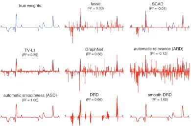
Fig. 3 shows an example weight vector drawn from this prior, along with estimates obtained from a variety of different estimators:
• lasso (Tibshirani, 1996), using Least Angle Regression (LARS) implemented by
glm-net1;
true weights
(RTV-L12 = 0.59) (R2 = 0.50) GraphNet
(R2 = 1.00)
automatic smoothness (ASD)
(R2DRD = 0.66) smooth-DRD(R2 = 1.00)
(Rlasso2 = 0.03)
(R2 = -0.12) automatic relevance (ARD)
(RSCAD2 = -0.01)
Figure 3: Example 4000-element weight vectorwsampled from the smooth-DRD prior
(up-per left), and estimates obtained from different methods on a simulated dataset
withn= 500 samples. The R2 performance of each estimate in recoveringw is
indicated above each plot. The bottom row shows our estimators: DRD-Laplace (bottom center) and smooth-DRD-Laplace (bottom right); the other DRD and smooth-DRD estimators (not shown) achieved similar performance.
• Automatic Relevance Determination (ARD) (Neal, 1995; MacKay, 1992), implemented
with the classic fixed point algorithm.
• Automatic Smoothness Determination (ASD) (Sahani and Linden, 2003), which uses
numerical optimization of marginal likelihood to learn the hyperparameters of a
squared exponential kernel governing w.
• Total Variation l1 (TV-L1) (Michel et al., 2011; Baldassarre et al., 2012; Gramfort
et al., 2013), combining total variation penalty (also known as fused lasso), which imposes anl1 penalty on the first-order differences ofw, with a standard lasso penalty.
• GraphNet (Grosenick et al., 2011), a graph-constrained elastic net, developed for
spatial and temporally correlated data that yields interpretable model parameters by incorporating sparse graph priors based on model smoothness or connectivity, as well as a global sparsity inducing a prior that automatically selects important variables.
• Smoothly Clipped Absolute Deviation (SCAD) (Fan and Li, 2001), an estimator with
We computed total variation l1 (TV-L1) and graph net (GraphNet) estimates using the
Nilearn2 package (Abraham et al., 2014). SCAD was implemented by SparseReg3 (Zhou
and Gaines, 2017). For lasso, GraphNet, TV-L1 and SCAD, we used cross-validation to set hyperparameters, whereas ARD and ASD used evidence optimization to automatically set hyperparameters. For the DRD estimators, we used evidence optimization to set hyperpa-rameters for Laplace-approximation based estimates and used sampling to integrate over hyperparameters for MCMC-based estimates.
For the basic DRD model, which incorporates structured sparsity but not smoothness, we compared three different inference methods: (1) Laplace approximation based infer-ence (“DRD-Laplace”); (2) Markov Chain Monte Carlo (“DRD-MCMC”); and (3) Convex relaxation based optimization (“DRD-Convex”). Lastly, for the smooth-DRD model, we used two inference methods: (4) Laplace approximation (“smooth-DRD-Laplace”); and (5) MCMC (“smooth-DRD-MCMC”). For the non-MCMC estimators, we initialized the
vector of Fourier domain coefficients ˜v (eq. 49) to values of 10−3 in the first iteration
when learning u. The hyper-hyperparameters in the MCMC methods (eq. 47) were set to:
mn=−2, σn2 = 5, mb =−10, σb2= 8, aρ= 4, bρ= 5, al = 4, bl = 25, aδ= 4, bδ = 25.
Fig. 3 shows the reconstruction performance (R2) of the true regression weight w for
dif-ferent estimators. The reconstruction performance metric for an estimate ˆw is given by
R2 = 1− ||w−wˆ||22 ||w−w¯||2 2
, where || · ||2 denotes the l2-norm and ¯w = 1pPpi=1wi is the mean of
vectorw. The true weight vector was sampled from the smooth DRD model. The
smooth-DRD estimate achieved the best performance in terms of R2. The ASD estimate also
performed well, although the estimate was not sparse, exhibiting small wiggles where the
coefficients should be zero. The standard DRD estimate recovered the support of w with
high accuracy, but had larger error than smooth-DRD estimates due to the smoothness of
the truew. The other methods (lasso, ARD, TV-L1, GraphNet and SCAD) all had lower
accuracy in recovering both the support and values of the regression weights.
To provide insight into the performance of ARD, DRD, and smooth-DRD, we plotted the inferred prior covariance of each model (Fig. 4). The DRD and smooth-DRD models were both similar to ARD in that they achieved sparsity by shrinking the prior variance of un-necessary coefficients to zero. However, unlike ARD, their inferred prior covariances both exhibited clusters of non-zero coefficients, reflecting the dependencies introduced by the latent Gaussian process. Note also that ARD and DRD covariances were both diagonal, making the weights independent given the prior variances, whereas the smooth-DRD co-variance had off-diagonal structure that induced smoothness.
To quantitatively validate that our estimators succeed at identifying structured sparse and smooth structure, we performed simulated experiments using data drawn from the DRD
generative model. For each experiment, we generated simulated data withn= 500 samples
from a p-element weight vector, and varied p from 500 to 4000. We used hyperparameters
GP mean b = −8, GP length scale l = p/40, GP marginal variance ρ = 36, smoothness
length scale δ = p/20, and varied measurement noise variance σ2 between 1 and 50. The
sparsity ratio for the sampled weights w was approximately 0.20, where we considered
ARD DRD smooth-DRD
Figure 4: Estimated filter weights and prior covariances. The upper row shows the true filter (blue) and estimated ones (red); the middle row displays the diagonal of each estimated covariance matrix; and the bottom row shows the entire estimated covariance matrix for each prior.
weights with |wi|>0.005 to be non-zero. We varied training set size fromn= 100 to 400
and kept a fixed test size of 100 samples. (We noted that even with n= 400 samples, the
problem resides in the n < psmall-sample regime). We repeated each experiment 5 times.
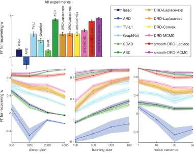
We compared performance of DRD estimators to the above-mentioned estimators. Fig. 5
shows the reconstruction performance (R2) of the true regression weights w for different
estimators as a function of noise variance, training set size and dimension.
We found that Laplace and MCMC estimates for the smooth-DRD model outperformed other estimators and were approximately equally accurate, indicating that use of Laplace approximation did not noticeably harm performance relative to the fully Bayesian estimate. ASD had a good performance indicating that for these extremely smooth weights, smooth-ness was a more useful form of regularization than structured sparsity conferred by DRD. DRD models came next. DRD-MCMC was slightly better due to the robustness of the fully Bayesian inference. DRD-Laplace-exp and DRD-Convex employed the exponential
nonlin-earity when transforming u to the diagonal of the covariance matrix. DRD-Laplace-rec
used a soft-rectifier nonlinearity which was more numerically stable. They had similar R2
values with TV-L1 when recoveringw, but were better than all the other methods. We can
also investigate the influence of each variable, i.e. noise variance, training size or
dimen-sion. When increasing the noise variance, all theR2 values dropped; smooth-DRD-MCMC
outperformed others with σ2 = 50 indicating the power of the fully Bayesian estimate and
All experiments
lasso ARD TV-L1 GraphNet SCAD ASD
DRD-Laplace-exp DRD-Laplace-rec DRD-Convex DRD-MCMC smooth-DRD-Laplace smooth-DRD-MCMC 0
1
lasso
GraphNet
SCAD
ASD
smooth-DRD-Laplac
ARD
TV
-L1
DRD-Laplace-exp DRD-Laplace-rec DRD-Convex
DRD-MCMC smooth-DRD-MCMC
R for recovering w
2
-0.4 0 0.4 0.8
-0.4 0 0.4 0.8
-0.4 0 0.4 0.8
500 1000 2000 4000
dimension 100 200training size300 400 1 noise variance10 30 50
R for recovering w
2
Figure 5: Comparison of performance recovering true regression weights w in simulated
experiments as a function of dimensions p (lower left), number of samples n
(lower middle), and noise variance σ2 (lower right). Experiments were repeated
five times for each of 64 combinatorial settings of four values for p, n, and σ2.
Traces show averageR2 (±1 standard error of the mean (SEM)) as a function of
each variable, and the bar plot (top row) shows average R2 (±1 SEM) over all
5×64 = 320 experiments.
and were comparable with DRD-MCMC, which was due to the decreasing optimizing com-plexity. Also surprisingly, smooth-DRD estimators achieved nearly perfect reconstruction performance over all the training sizes and all the dimensions.
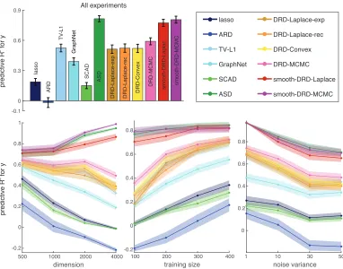
Fig. 6 shows the R2 performance for regression prediction on the test set for different
estimators as a function of noise variance, training set size and dimension. The reconstruc-tion performance for recovering the true ytest is given by R2 = 1− ||ytest−yˆtest||22
||ytest−y¯test||2 2
, where ¯
ytest = ntest1
Pntest
i=1 ytest,i is the mean of vector ytest. The top-left subfigure presents the
averaged R2 values and the confidence intervals for ˆytest over all runs. Similar to R2 for
w, ASD estimate, Laplace and MCMC estimates for the smooth-DRD model outperformed
All experiments
predictive R for y
2
-0.1 0 0.3 0.6 0.9
lasso
GraphNet
SCAD ASD
smooth-DRD-Laplac
ARD
TV
-L1
DRD-Laplace-exp DRD-Laplace-rec DRD-Convex
DRD-MCMC smooth-DRD-MCMC
500 1000 2000 4000
dimension -0.2
0 0.2 0.4 0.6 0.8 1
100 200 300 400
training size -0.2
0 0.2 0.4 0.6 0.8
1 10 30 50
noise variance 0
0.2 0.4 0.6 0.8 lasso ARD TV-L1 GraphNet SCAD ASD
DRD-Laplace-exp DRD-Laplace-rec DRD-Convex DRD-MCMC smooth-DRD-Laplace smooth-DRD-MCMC
predictive R for y
2
Figure 6: Comparison of performance predicting held-out responses ytest in simulated
ex-periments as a function of dimensionsp (lower left), number of samplesn(lower
middle), and noise varianceσ2 (lower right). Traces show averageR2 (±1 SEM),
and the bar plot (top row) shows average R2 (±1 SEM) over all experiments.
Simulation experiments were the same as in Fig. 5.
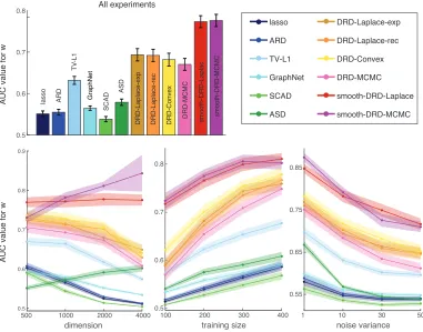
Fig. 7 shows the AUC (Area Under the receiver operator characteristic Curve) values for different estimators as a function of noise variance, training set size and dimension. The
AUC metric quantifies accuracy in recovering the binary support for w, which is useful for
assessing the effects of structured sparsity. For this metric, the smooth DRD estimators outperformed other methods, and the ASD estimator performed much worse due to its lack of sparsity. The Laplace approximation based DRD models performed slightly better than DRD-MCMC because the sparsity of MCMC estimates was diluted by averaging across multiple samples.
Overall, smooth-DRD outperformed all other methods using all metrics. This shows that combining sparsity and smoothness can provide major advantages over methods that impose
only one or the other. This flexible framework for integrating structured sparsity and
All experiments
lasso ARD TV-L1 GraphNet SCAD ASD
DRD-Laplace-exp DRD-Laplace-rec DRD-Convex DRD-MCMC smooth-DRD-Laplace smooth-DRD-MCMC
0.5 0.6 0.7 0.8
lasso GraphNet
SCAD
ASD
smooth-DRD-Laplac
ARD
TV
-L1
DRD-Laplace-exp DRD-Laplace-rec DRD-Convex DRD-MCMC smooth-DRD-MCMC
AUC value for w
AUC value for w
0.5 0.6 0.7 0.8 0.9
0.5 0.6 0.7 0.8
0.55 0.65 0.75 0.85
500 1000 2000 4000
dimension 100 200training size300 400 1 noise variance10 30 50
Figure 7: Comparison of performance at recovering support of regression weights in simu-lated experiments, quantified with area under the ROC curve (AUC), as a
func-tion of dimensionsp (lower left), number of samplesn (lower middle), and noise
varianceσ2 (lower right). Traces show averageAU C (±1 SEM), and the bar plot
(top row) shows average AU C (±1 SEM) over all experiments. Simulation
ex-periments were the same as in Fig. 5. Support recovery was quantified by taking all coefficients|wi|>0.005 as non-zero.
in the structured sparsity literature which consider only sparsity. The code and simulated results are available online4.
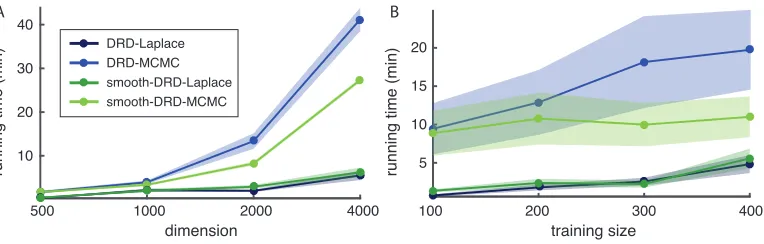
5.2. Computational complexity and optimization
We have described two basic approaches to inference for DRD: evidence optimization using the Laplace approximation and MCMC sampling-based inference. The main computational difficulty associated with Laplace-based methods is the Hessian matrix, which provides
the precision matrix for the approximate Gaussian posterior distribution. This matrix
costs O(p2) to store and contributes O(p3) time complexity for computation of the
0 0 0 4 0 0 0 2 0 -2 2 6 0 0 0 4 0 0 0 2 0 -2 2 6 0 0 0 4 0 0 0 2 0 -2 2 6 0 0 0 4 0 0 0 2 0 -2 2 6 0 0 0 4 0 0 0 2 0 -2 2 6 0 0 0 4 0 0 0 2 0 -2 2 6 0 0 0 4 0 0 0 2 0 -2 2 6 0 0 0 4 0 0 0 2 0 -2 2 6 0 0 0 4 0 0 0 2 0 -2 2 6 0 0 0 4 0 0 0 2 0 -2 2 6 0 0 0 4 0 0 0 2 0 -2 2 6 0 0 0 4 0 0 0 2 0 -2 2 6 DRD-Laplace DRD-Convex DRD-Laplace DRD-Convex iteration
0 20 40 60 80
0 5 10 15 20 25 30 iter 5 10 20 50 100 200
Figure 8: Comparison of the optimization of weights ˆw between Laplace and
DRD-Convex. The first two columns show the weights obtained after 5, 10, 20, 50, 100, and 200 iterations with the same initialization under the two estimators, with true weights indicated in black. The third column shows the change in weights after each iteration of the standard and convex optimization algorithms over the first 80 iterations, showing that the convex algorithm made much smaller adjustments to the weights after the first few iterations and thus converged more rapidly.
running time (min)
running time (min)
A B
5 10 15 20
100 200 300 400
training size 10
20 40
30
500 1000 2000 4000
dimension
DRD-MCMC smooth-DRD-Laplace smooth-DRD-MCMC DRD-Laplace
Figure 9: Running times for DRD estimators as a function of dimensionsp(left) and
num-ber of samples n (right). Each point is an average across 20 simulated
experi-ments, and the shaded area represents ±1 SEM. For MCMC, running time was
determined by the time to collect 100 posterior samples after burn-in.
We also described a two-step convex relaxation of the Laplace method (DRD-Convex), which takes more time per iteration than the standard Laplace method (DRD-Laplace) due to the need for a two-step optimization procedure. However, we find that the DRD-Convex takes fewer iterations to converge (see Fig. 8), and in some cases proves more successful at avoiding sub-optimal local optima.
The MCMC-based inference has a time complexity of only O(n2pf) per sample, due to the
fact that there is no need to compute the Hessian. However, MCMC-based inference is typ-ically slower due to the need for a burn-in period and the generation of many samples from the posterior. Fig. 9 shows a comparison of running time for the two inference methods for both DRD and smooth-DRD models. For the Laplace method, we used a stopping criterion
that the change in w was less than 0.0001. For the MCMC method, we assessed burn-in
using a criterion on the relative change inw, and then collected 100 posterior samples.
In-ference for the smooth-DRD model was faster than for standard DRD due to the fact that the smoothing prior effectively prunes high frequencies, reducing the dimensionality of the
search space forw. In these experiments, increasing dimensionpelicited larger increases in
computation time than increasing training set size n.
6. Phase transition in sparse signal recovery
Compressive sensing focuses on the recovery of sparse high-dimensional signals in settings
where the number of signal coefficients p exceeds the number of measurements n. Recent
work has shown that the recovery of sparse signals exhibits a phase transition between perfect and imperfect recovery as a function of the number of measurements (Ganguli and
Sompolinsky, 2010; Amelunxen et al., 2014). Namely, when the measurement fraction
γ = n/p exceeds some critical value that depends on signal sparsity, the signal can be
recovered perfectly with probability approaching 1, whereas forγbelow this value, estimates
contain errors with probability approaching 1. However, these results were derived for the case where non-zero coefficients are randomly located within the signal vector. Here we
show that DRD can obtain dramatic improvements over the phase transition curve for iid
sparse signals when the non-zero coefficients arise in clusters.
We performed simulated experiments to examine the effects of group structure on the em-pirical phase transition between perfect and imperfect recovery of sparse signals. The mea-surement equation is given by the noiseless version of the linear system we have considered
so far: y =Xw, where w ∈ Rp is the sparse signal, y ∈ Rn is the (dense) measurement
vector, and hereX∈Rn×p is a (short, fat) random measurement matrix with entries drawn
iid from a standard normal distribution. We define the sparsity of the signal as α =k/p,
wherek is the number of non-zero signal coefficients inw.
To explore the effects of group structure, we considered the signal coefficients in w to
have 1D spatial structure and introduced a parameter g specifying the number of spatial
groups or clusters into which the non-zero coefficients were divided. When g = 1, the
non-zero coefficients formed a single contiguous block of lengthk, with location uniformly
distributed within w. When g > 2, the non-zero coefficients were divided intog blocks of
lasso DRD, g=1 DRD, g=2 DRD, g=3 DRD, g=4 DRD, g=10 sDRD, g=1 sDRD, g=2 sDRD, g=3 sDRD, g=4 sDRD, g=10 lasso
DRD, g=1 DRD, g=2 DRD, g=3 DRD, g=4 DRD, g=10 m
e
a
su
re
m
e
n
t
ra
te
structured sparse smooth structured sparse
m
e
a
su
re
m
e
n
t
ra
te
sparsity level sparsity level
0 250 500
-2 0 2 4
0 250 500
-2 0 2 4
Figure 10: Phase transitions for DRD and smooth-DRD (sDRD) estimators on
signals with structured sparsity. Top row shows example signals w of
di-mensions p = 500, which contain randomly positioned blocks of non-zero
co-efficients. Non-zero coefficients were clustered into varying numbers of groups
g, and drawn either iid from a standard normal distribution (left column) or
from a Gaussian with a smoothing kernel (length scale was 20) (right column), to illustrate the effects of smoothness. To compute phase transition curves, we analyzed the recovery behavior of each estimator at every point in a 2D grid of
sparsity levelsα and measurement ratesγ. At each point, we generated 10
ran-dom signalsw, projected them noiselessly onto a random Gaussian measurement
matrixX, and computed lasso and DRD estimates ˆw. We then calculated the
R2 value of the estimates for each trial at every grid point (α, γ). An estimator was considered to achieve perfect recovery if all 10 trials resulted inR2 >0.95, and perfect failure if all 10 trials resulted inR2 ≤0.95; remaining points were considered to fall in the phase transition region. For each estimator, the shaded region indicates the phase transition region, and solid line indicates its center of mass along the y-axis.
the constraint that blocks remained disjoint. Once the sparsity pattern was determined, we sampled the non-zero coefficients from a standard normal distribution.
Fig. 10 shows the empirical phase transition curves for lasso and DRD estimators for sparse
show the boundary between perfect and imperfect signal recovery for different estimators
in the 2D space of signal sparsity level α and measurement fraction γ. The left bottom
plot shows that DRD estimators achieved perfect signal recovery for much lower measure-ment rates, even when non-zero coefficients were clustered into as many as 10 groups. Here DRD achieved transition to perfect recovery along the main diagonal, whereas lasso exhib-ited an arc-shape transition curve described previously (Ganguli and Sompolinsky, 2010; Amelunxen et al., 2014), indicating that more measurements were required to recovery signals of equal sparsity. In the right bottom plot, we generated the non-zero coefficients from a Gaussian distribution with a smoothing kernel whose length scale equaled to 20, so that non-zero coefficients were smooth as well as sparse. In these plots, we compared lasso estimates (which do not benefit from group or smooth structure) to standard DRD and smooth-DRD estimates. This reveals that smoothness allows for further reductions in mea-surement rates, with perfect signal recovery achievable well below that of the non-smooth DRD estimates.
7. Applications to brain imaging data
Functional magnetic resonance imaging (fMRI) measures blood oxygenation levels, which provide a proxy for neural activity in different parts of the brain. Although these mea-surements are noisy and indirect, fMRI is one of the primary non-invasive methods for measuring activity in human brains, and it has provided insight into the neural basis for a wide variety of cognitive abilities and functional pathologies.
A primary problem of interest in the fMRI literature is “decoding”, which involves the use of linear classification and regression methods to identify the stimulus or behavior associated with measured brain activity. Decoding is a challenging statistical problem because the number of volumetric pixels or “voxels” measured with fMRI is typically far greater than the number of trials in an experiment; a full brain volume typically contains 50K voxels whereas most experiments produce only a few hundred observations.
Standard approaches to decoding have therefore tended to exploit sparsity, corresponding to the assumption that only a small set of brain voxels are relevant for decoding a particular set of stimuli (Carroll et al., 2009). However, the set of voxels useful for a specific decoding task are not randomly distributed throughout the brain, but tend to arise in clusters; if
one voxel carries information useful for decoding, it isa priorilikely that nearby voxels do
too, given that voxels represent an arbitrary discretization of continuous underlying brain structures. We therefore explored brain decoding as an ideal application for evaluating the performance of our estimators.
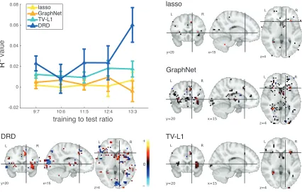
7.1. Gambling task
pre-lasso
GraphNet
0 +
-TV-L1 DRD
training to test ratio
r
2 value
-0.02 0 0.02 0.04 0.06
0.08 lasso
GraphNet TV-L1 DRD
R
9:7 10:6 11:5 12:4 13:3
Figure 11: Top left panel shows average testR2 values on the gambling dataset as a function
of the train-test ratio for lasso, GraphNet, TV-L1 and DRD. The x-axis is the
train-test split ratio and the y-axis is the R2 criterion. The remaining panels
show the estimated fMRI weight maps, overlaid on a structural fMRI image. Colors indicate the sign and magnitude of the weights (see color bar, red for positive, blue for negative, black for small). The DRD figure was obtained by cutting off small weight coefficients with a small threshold value at 0.004 (about 12% of the maximal absolute coefficient value).
sented for 3s, and the participants were instructed to decide whether to accept or reject the gamble. Experimenters varied amount of the potential gain and loss across trials. The regression task is to predict the gain of the gamble from the fMRI images recorded during the decision-making task.
After standard preprocessing, the regression dataset consisted of 16 subjects with 48 fMRI measurements per subject (resulting from 6 repeated presentations of 8 different gambles).
fMRI measurements were obtained from a 3D brain volume of 40×48×34 voxels, each of size
4×4×4 mm, from which a subset of 33,177 valid brain voxels were used for analysis. The
full dataset of 16 subjects therefore containedn= 768 samples in ap= 33,177 dimensional
space.
held-out subjects. To assess the performance, we varied the train-test ratio in number of subjects from 9:7 to 13:3. We performed 10 different random train-test splits for each ratio. We used 5-fold cross-validation to set hyperparameters for all models, including DRD. For DRD models, the Laplace approximation was intractable due to the high dimensionality of
the weight vector (p= 33,177). We therefore computed MAP estimates of the latent vector
u conditioned on the hyperparameters, and set hyperparameters using cross-validation.
The curves in the top left panel of Fig. 11 show the performance of lasso, GraphNet, TV-L1 and DRD estimators. We found that DRD outperformed other estimators at nearly all train-test ratios, with a noticeable advantage at the largest training set size. However, we noted that the SNR of this dataset was low, making inter-subject prediction difficult and resulting in low accuracy for all methods. A non-trivial preprocessing stage, such as hyper-alignment (Chen et al., 2015), could be used to map different subjects into a shared subspace, which reduces the low SNR induced by inter-subject variability and could possibly improve performance.
Fig. 11 also shows the inferred regression weights for each estimator. The GraphNet and lasso weights had high sparsity, presumably due to the low SNR of the dataset, while TV-L1 weights exhibited small blocks of non-zero coefficients with constant value within each block, consistent with the structure expected for the TV-L1 penalty. The DRD weights were not sparse in a strict L0 sense, due to the fact that sparsity arises from soft-rectification of negative latents governing the prior variance. We therefore thresholded DRD weights for plotting purposes, revealing that the weights contributing most to prediction performance tended to cluster, as expected, although weights within each cluster were not constant. One noteworthy observation is that DRD estimate had positive (red) as well as negative weights (blue), while other estimates were largely devoid of regions with negative weights. Note that voxels in black indicate weights close to zero, which therefore contributed relatively little to readout.
7.2. Age prediction task
Next we considered the problem of predicting a subject’s age from a measured map of gray-matter concentration, using data from the Open Access Series of Imaging Studies (OASIS) (Marcus et al., 2007). The OASIS dataset consisted of T1-weighted MRI scans data from 403 subjects aged 18 to 96, with 3 or 4 scans per subject. One hundred of these subjects were over 60 years of age and had been clinically diagnosed with Alzheimer’s. The repeated scans provided high signal-to-noise ratio, making the dataset feasible for inter-subject analyses.
A natural regression problem for this dataset is to predict the age of subject from their
anatomical MRI data. The full dataset consisted of 403 samples with a 91×109×91 3D
volume and 129,081 valid voxels. To assess the performance, we varied the training ratio from 0.4 to 0.8 out of the 403 subjects, and averaged over 5 random splits for each ratio.
The curves in the top left panel of Fig. 12 show mean absolute errors between the true age and the predicted age for each estimator, evaluated on test data. The DRD and smooth-DRD estimators, which performed similarly well, achieved lower error than lasso, GraphNet,