Thompson Sampling Guided Stochastic Searching on the
Line for Deceptive Environments with Applications to
Root-Finding Problems
∗Sondre Glimsdal [email protected]
Centre for Artificial Intelligence Research (CAIR)
University of Agder Postboks 422, 4604 Kristiansand, Norway
Ole-Christoffer Granmo [email protected]
Centre for Artificial Intelligence Research (CAIR)
University of Agder Postboks 422, 4604 Kristiansand, Norway
Editor:Avi Pfeffer
Abstract
The multi-armed bandit problem forms the foundation for solving a wide range of online stochastic optimization problems through a simple, yet effective mechanism. One simply casts the problem as a gambler who repeatedly pulls one out of N slot machine arms, eliciting random rewards. Learning of reward probabilities is then combined with reward maximization, by carefully balancing reward exploration against reward exploitation. In this paper, we address a particularly intriguing variant of the multi-armed bandit problem, referred to as theStochastic Point Location (SPL)problem. The gambler is here only told whether the optimal arm (point) lies to the “left” or to the “right” of the arm pulled, with the feedback being erroneous with probability 1−π. This formulation thus targets optimization in continuous action spaces with both informative and deceptive feedback. To tackle this class of problems, we formulate a compact and scalable Bayesian represen-tation of the solution space that simultaneously captures both the location of the optimal arm as well as the probability of receiving correct feedback. We further introduce the ac-companying Thompson Sampling guided Stochastic Point Location (TS-SPL) scheme for balancing exploration against exploitation. By learningπ, TS-SPL also supportsdeceptive environments that are lying about the direction of the optimal arm. This, in turn, allows us to address the fundamental Stochastic Root Finding (SRF) problem. Empirical results demonstrate that our scheme deals with both deceptive and informative environments, significantly outperforming competing algorithms both for SRF and SPL.
Keywords: thompson sampling, searching on the line, probabilistic bisection search, deceptive environment, stochastic point location
1. Introduction
Research on the Stochastic Point Location (SPL) problem (Oommen, 1997) has delivered increasingly efficient schemes for locating the optimal point on a line. In all brevity, the optimal point must be found based on iteratively proposing candidate points, with each candidate revealing whether the optimal point lies to the candidate’s left or to its right. The provided directions can be erroneous, and the goal is to locate the optimal point with
∗. A preliminary version of some of the results of this paper appears in the Proceedings of AIAI’15.
c
as few non-optimal candidate proposals as possible. The SPL problem can also be cast as an agent that moves on a line, attempting to locate a particular location λ∗. The agent communicates with a teacher that notifies the agent whether its current locationλis greater or lower thanλ∗. However, the teacher is of a stochastic nature and feeds the agent erroneous feedback with probability 1−π.
Despite the simplicity of the SPL problem, SPL schemes have provided novel solu-tions for a wide range of problems. Intriguing applicasolu-tions include the estimation of non-stationary binomial distributions (Yazidi et al., 2012b), communication network routing (Oommen et al., 2007), and meta-optimization (Oommen et al., 2009). Furthermore, re-cent research that addresses the related Stochastic Root-Finding (SRF) problem provides promising solutions for parameter estimation, transportation system optimization, as well as supply chain optimization (Chen and Schmeiser, 2001; Pasupathy and Kim, 2011).
State-of-the-art. Adaptive Step Searching (ASS) (Tao et al., 2013) is currently the leading approach to solving SPL problems, although it is outperformed by Hierarchical Stochastic Searching on the Line (HSSL) (Yazidi et al., 2012a) in highly volatile non-stationary environments (Tao et al., 2013). Optimal Computing Budget Allocation (OCBA) has also been applied to SPL (Zhang et al., 2015) and provides stable solutions while con-verging slightly slower than ASS. Unfortunately, these state-of-the-art schemes fail when noise increases beyond a certain degree, which happens when the majority of obtained direc-tions mislead rather than guide. Indeed, by naively following the direcdirec-tions provided under such circumstances, one is systematically led away from the optimal point. We refer to these kinds of problem environments as deceptiveenvironments, as opposed to informative ones, which are explained in more detail below.
To the best of the authors’ knowledge, the pioneering CPL-AdS (Oommen et al., 2003) scheme was the first known approach handling deceptive SPL environments. CPL-AdS relies on two consecutive phases. In the first phase, a sequence of intelligently selected questions is used to classify the environment as either informative or deceptive. By spending a sufficient amount of time in this phase, the classification can be made arbitrarily accurate. In the second phase, a regular SPL scheme is applied, except that the directions obtained are reversed if the problem environment was classified as deceptive in the first phase. This means that the scheme may have to remain in the first phase for an extensive amount of time to ensure that the problem environment is correctly classified, otherwise, one risks being systematically misled in the second phase. These properties largely render CPL-AdS inappropriate for online or anytime problem solving.
Recently, HSSL has been extended by Zhang et al. to cover both informative and de-ceptive environments, using a Symmetric HSSL (SHSSL) scheme (Zhang et al., 2016). This scheme essentially runs two HSSL schemes in conjunction: one regular, which handles in-formative environments, and one that inverts all feedback from the environment, to handle deceptive environments. The hierarchy navigation capabilities of HSSL are then exploited to allow SHSSL to switch between the two HSSLs, depending on the nature of the environ-ment. However, a significant limitation of HSSL, namely, that π must be larger than the conjugate of the golden ratio, carries over to SHSSL. Indeed, SHSSL fails to converge for
et al., 2003), since both of these schemes operate along the whole range of π (apart from
π= 0.5).
To cast further light on the challenges lined out above, we here introduce the N-Door Puzzle as a framework for modeling deception. We also propose an accompanying novel solution scheme — Thompson Sampling guided Stochastic Point Location (TS-SPL). The TS-SPL scheme handles both SPL and SRF problems, and is capable of simultaneously solving the problem as well as determining whether we are dealing with an informative or a deceptive environment. As we shall see, not only does this scheme handle an arbitrary level of noise, but it also outperforms current state-of-the-art techniques in both informative and deceptive environments.
The N-Door Puzzle. In the book ”To Mock a Mockingbird” (Smullyan, 1988) the following puzzle is formulated: ”Someone was sentenced to death, but since the king loves riddles, he threw this guy into a room with two doors. One leading to death, one leading to freedom. There are two guards, each one guarding one door. One of the guards is a perfect liar, the other one will always tell the truth. The man is allowed to ask one guard a single yes-no question and then has to decide, which door to take. What single question can he ask to guarantee his freedom?” To avoid spoiling the puzzle for the reader, we omit the solution here and note that asking a double negative question will often be the correct course of action for these types of puzzles.
The above puzzle can be generalized by increasing the number of doors. Instead of deciding between merely two doors, the prisoner now faces N doors, with a guard posted between each pair of doors. Only a single door leads to freedom, the remaining doors lead to death. Every day at sunrise, the prisoner is allowed to ask one of the guards whether the door leading to freedom is to the left or to the right of the guard. However, only a fixed proportion of the guards answers truthfully, the rest are compulsive liars. Further, the guards are randomly assigned a position at each sunrise, and thus, knowing who lies and who tells the truth is impossible. As an additional complication, depending on the mood of the king, the prisoner may be ordered to walk through a door of his choice at an arbitrary day. Therefore, to save his life, it is imperative that the prisoner determines as quickly as possible which door leads to freedom.
Specifically, let π = #truthful guards#guards be the fraction of truthful guards. Since the guards are randomly assigned a position each day, the probability of obtaining a truthful answer is governed by π. If π < 0.5 then the majority of the guards are compulsive liars, and the guards as an entity can be characterized as beingdeceptive. Conversely, ifπ >0.5 then the majority of the guards are truthful and the guards can be seen as informative. For completeness, we mention that the puzzle is unsolvable for the case whereπ is exactly equal to 12, since it is then impossible to obtain any information on neither the nature of the doors nor the guards.
these probabilities are unknown to the decision maker. The challenge is thus to decide which of the arms to pull at each time step, to maximize the expected total number of rewards obtained (Bubeck and Cesa-Bianchi, 2012).
In all brevity, TS seeks to achieve the above goal by quickly shifting from exploring reward probabilities to maximizing the number of rewards obtained. This is achieved by recursively estimating the underlying reward probability of each arm, using Bayesian filter-ing of the rewards obtained so far. TS then simply selects the next arm to pull based on the Bayesian estimates of the reward probabilities (one reward probability density function per arm).
The arm selection strategy of TS is rather straightforward, yet surprisingly efficient. To determine which arm to pull, a single candidate reward probability is sampled from the probability density function of each arm. The arm with the highest sample value is the one pulled next. The outcome of pulling this arm is in turn used to perform the next Bayesian update of the arm’s reward probability estimate. It is this simple scheme that makes TS select arms with frequency proportional to the posterior probability of being optimal, leading to quick convergence towards always selecting the optimal arm.
TS has turned out to be among the top performers for traditional MAB problems (Granmo, 2010; Chapelle and Li, 2011), supported by theoretical regret bounds (Agrawal and Goyal, 2012, 2013a; Dong and Van Roy, 2018). It has also been successfully applied to contextual MAB problems (Agrawal and Goyal, 2013b), constrained Gaussian process optimization (Glimsdal and Granmo, 2013), distributed quality of service control in wireless networks (Granmo and Glimsdal, 2013), cognitive radio optimization (Jiao et al., 2016), as well as a foundation for solving the maximum a posteriori estimation problem (Tolpin and Wood, 2015).
Pure Exploration Bandits. Throughout this paper we assume that each SPL prob-lem potentially takes part in a larger system consisting of multiple SPL probprob-lems, and not necessarily operating in isolation. From existing applications in the literature, such as web crawler load balancing (Granmo et al., 2007), it is clear that the value of an SPL scheme does hinge upon its ability to cooperate and interact with other decision makers. Such cooperation demands predictable behaviour from the individual decision makers, as well as coordinated balancing of exploring new solution candidates against maintaining good solution candidates. Without such an ability, the system as a whole will not be able to sys-tematically move towards the more promising areas of the search space, gradually focusing in on an optimal configuration. Therefore, in this paper we omit a direct comparison with schemes that rely on a ”fixed sampling then decide” approach, such as unimodal bandits (Jia and Mannor, 2011). For the same reason, we will not investigate purely exploitative bandits (Even-Dar et al., 2006; Jamieson et al., 2014; Audibert and Bubeck, 2010; Gabillon et al., 2011; Karnin et al., 2013), bandits that have a predefined finite time horizon and whose performance is only measured at the end of that horizon. Such algorithms are free to explore without any negative impact, and this allows them to outperform traditional exploitation-exploration bandits such as TS and UCB in scenarios where exploitation is not required.1
Paper Contributions. In this paper, we introduce a novel scheme for solving the SPL problem, namely, TS-SPL. At the core of TS-SPL, we find a compact and scalable Bayesian representation of the SPL solution space. This Bayesian representation simultaneously cap-tures both the location of the optimal point (bandit arm) as well as the probability of receiving correct feedback. We further introduce an accompanying scheme for balancing exploration against exploitation, based on TS. By learning π, TS-SPL also supports de-ceptive environments that are lying about the direction of the optimal arm. This, in turn, allows us to solve the fundamental SRF problem. More specifically, the contributions of the paper can be summarized as follows:
1. We introduce a novel TS-SPL scheme that represents the solution space of N-Door Puzzles, and thus SPL problems, in terms of a Bayesian model. As opposed to compet-ing solutions that merely maintain and refine a scompet-ingle candidate solution, our Bayesian model encompasses the complete space of candidate solutions at every time instant.
2. We formulate a compact and scalable Bayesian representation of the solution space that simultaneously captures both the location of the optimal point (arm), as well as the probability of receiving correct feedback. This Bayesian representation of the problem opens up for efficient exploration and exploitation of the solution space with TS.
3. We link TS-SPL to so-called stochastic bisection search; and unify accompanying methods under the umbrella of TS.
4. Similarly, we enhance the Soft Generalized Binary Search (SGBS), Probabilistic Bisec-tion Search (PBS) and Burnashev-Zigangirov Algorithm (BZ) by introducing novel parameter free solutions that take advantage of our Bayesian model of the N-door puzzle and the SPL problem. This approach eliminates previous reliance on knowing the exact degree of noise affecting the system to be optimized.
5. We provide the first unified empirical comparison of the key state-of-the-art SPL- and SRF solvers.
6. We finally demonstrate the empirical performance of TS-SPL for both SPL and SRF problems. TS-SPL outperforms the state-of-the-art algorithms in both informative and deceptive environments, except for the SGBS and BZ schemes with correctly specified observation noise.
Paper Outline. The paper is organized as follows. In Section 2, we present our scheme for TS guided SPL (TS-SPL). We first introduce the Bayesian model of the N-door puzzle. Based on the Bayesian model, we then formulate our TS-based scheme that balances solution space exploration against reward maximization. We further extend selected state-of-the-art solution schemes with our Bayesian N-door puzzle model. This extension removes the need for knowing the observation noise beforehand. In Section 3, we provide extensive empirical results comparing TS-SPL with state-of-the-art schemes for both SPL and SRF. We conclude in Section 4 and point to promising directions for further work.
2. Thompson Sampling Guided Stochastic Point Location
In this section, we introduce the TS-SPL scheme. The scheme can be summarized as follows. At the core of TS-SPL we find a Bayesian model of the N-Door Puzzle. Formally, we repre-sent an instance of the N-door puzzle as a tuple (λ∗, π∗)∈D×T, whereD={d1, . . . , dN}
is the set of doors andT ∈[0,1] is the truthfulness of the guards. Let (λ∗, π∗) be the partic-ular N-door puzzle faced. A novel aspect of TS-SPL is that instead of maintaining a single or a limited set of candidate solutions, we instead maintain a posterior distribution over the whole solution space, (λ, π) ∈D×T. This distribution is conditioned on the feedback already obtained up to time step n, allowing us to single in on (λ∗, π∗) as the number of time steps increases, ultimately converging to (λ∗, π∗).
Assuming no prior information, we assign a uniform distribution over D×T, i.e., all puzzle instances are equally probable. By gradually refining the posterior distribution over
D×T, we can select guards to question in a goal-oriented manner. In all brevity, we sample a solution candidate (λc, πc) from D×T, selecting the guard to the left or to right of λc. The answer of the selected guard is then used to update our posterior distribution. By repeating this procedure, the expected probability of the underlying N-door puzzle instance (λ∗, π∗) increases monotonically, reducing the probability of other puzzle instances. In effect, given enough iterations, TS-SPL will correctly identify the door leading to freedom as the posterior probability of (λ∗, π∗) approaches unity.
2.1 Bayesian Model of the N-Door Puzzle
The main purpose of the Bayesian model is to facilitate the efficient calculation of a posterior distribution over the possible N-door puzzle instances, D×T. Since the prisoner does not initially know which problem instance he is facing, and since the observations are stochastic, we castDandT as two random variables. We further assume thatDandT are independent of each other. Furthermore, the information we obtain from questioning the guards is represented as a set of random variables Q = {Q1, . . . , Qn}, with each random variable
Qk representing the answer from question k. Finally, we assume that the outcomes of the
individual questions Qk ∈ Q are independent when conditioned on D and P. For each questionQk, we can then compute the probability of the answer (”left” or ”right”) that we
received from the guard, as summarized in Table 1.
Guard to the left of door to freedom P(left|guard, door,t) =t P(right|guard, door, t) = 1−t
Guard to the right of door to freedom: P(left|guard, door,t) = 1−t P(right|guard, door, t) =t
Table 1: Conditional door probabilities
Applying Bayes Theorem to P(Q|d, t), defined in Table 1, we are able to derive closed-form expressions for the posterior distributions of bothDandT. The derivation ofP(d|Q),
d ∈ D, follows [the derivation of P(t|Q), t ∈ T, is analogous, and is left out here for the sake of brevity]:
P(d|Q) =X
t∈T
P(d, t|Q) (1)
∝X
t∈T
P(Q|d, t)P(d, t) (2)
=X
t∈T
P(Q|d, t)P(d)P(t) (3)
=X
t∈T
ˆ
QQ+P(d)P(t) (4)
Above, ˆQ = Qn−1
k=1P(Qk|d, t) and Q+ = P(Qn|d, t). Further, (2) follows directly from
Bayes Theorem. We obtain (3) as a result of the independence of D and T, and (4) from the independence between the questions inQ. This leads to the following two equations for updating our knowledge about both the door probabilities (5) and the truthfulness of the guards (6).
P(d|Q)∝X
t∈T
ˆ
QQ+P(d)P(t) (5)
P(t|Q)∝X
d∈D
ˆ
QQ+P(d)P(t) (6)
2.2 Guard Selection
We have now formally determined how we can transform information from the guards into a probability distribution over which door leads to freedom. However, as mentioned previously, we also face a trade-off between exploring different doors and zeroing in on the best door found so far. To handle this trade-off, we model the door selection as a so-called Global Information MAB (GI-MAB) (Atan et al., 2015).
To decide which door should be selected at each iteration, we solve the GI-MAB by utilizing the principle of TS. Here, the selection process is simply to select a random door proportional to the probability that this door is the one that leads to freedom. Once the door has been selected, we need to decide which of the guards to query: the guard to the left or to the right of the door selected. We do this by randomly selecting one of the guards, again proportional to the sum of the probabilities of the doors next to each guard. Let us assume for instance that we have three doorsdk,1≤k≤3 with the probabilities of leading
2.3 Improving State-of-the-Art Schemes with the Bayesian Model of the N-Door Puzzle
A main advantage of TS-SPL compared to similar schemes is the utilization of the Bayesian model that enables TS-SPL to operate without knowing the problem parameters in advance. Due to TS-SPL’s close connection to the Probabilistic Bisection Search (PBS) (Horstein, 1963), Noisy Generalized Binary Search (NGBS) (Nowak, 2008) and the BZ algorithm (Burnashev and Zigangirov, 1974), we will here use our Bayesian TS-SPL model to also make these other schemes parameter free.
Probabilistic Bisection Search
The goal of PBS2 (Waeber et al., 2013; Nowak, 2008) is to locate an unknown pointX∗ ∈
[0,1]. To acquire intelligence on the location of X∗, one queries an oracle of the relation between a point x and X∗. The oracle responds by informing whether x is on the left or the right side ofX∗. If we assume that the oracle is always telling the truth, then the well-known deterministic bisection search, which halves the search space with each query, can be employed to efficiently find X∗. However, in PBS we assume that the Oracle provides correct answers with probabilityp∈(0.5,1.0] and erroneous ones with probability 1−p.
The PBS can be traced back to Horstein (Horstein, 1963). In PBS a probability distribu-tion is mapped over the search space and is gradually updated using a Bayesian methodology under the assumption that the environment noisep is known a priori. The search space is then continuously explored using the median of the posterior distribution as the point of interest. It has been shown that PBS has a geometric rate of convergence under the latter assumptions (Waeber et al., 2013).
As the noisepis assumed to be given, one can simply invoke (7) to calculate the posterior distribution:
P(d|Q)∝P(Q|d)P(d). (7)
Here, P(Q | d) is the conditional probability of obtaining answer Q (point to the right). That is, for every location d to the left of X∗, the probability that the oracle directs the decision maker to the right is P(Q|d) =p. And conversely,P(Q|d) = 1−p fordto the right ofX∗.
To explicitly represent PBS’ dependence on knowing p beforehand, we can cast (7) in terms of (5) and (6). The resulting model is identical to TS-SPL, with the major difference that PBS employs the median to explore the search space. We denote this new and improved scheme PBS-M.
We also observe that due to its simple nature, PBS is particularly well-suited for parallel computing environments (Pallone et al., 2014), as opposed to more traditional stochastic approximation methods (Kushner and Yin, 1987).
PowerTest-Probabilistic Bisection Search
In a recent paper, Frazier et al. (Frazier et al., 2019) demonstrated an alternative approach to removing the dependency of PBS on knowing the fixed noise probability p. Instead of
applying a Bayesian prior overp, as done in TS-SPL, they introduce a frequency-based ap-proach, referred to as PowerTest-PBS (PT-PBS). PT-PBS is based on repeatedly sampling the underlying function g(x) until a pre-specified confidence α is archived on a hypothesis test over the sign of the feedback ofg(x). They further demonstrated that the asymptotic convergence of PT-PBS is similar to that of Stochastic Approximation (SA).
Generalized Binary Search
The Generalized Binary Search (GBS) problem can be formulated as follows (Nowak, 2008, 2011). Consider a collection of unique binary-valued functions H defined on a domain X. Each h ∈ H is defined as a mapping from X to {−1,1}. Assume that there exists an optimal function h∗ ∈ H that produces the correct binary labeling for each x ∈ X. For each queryx∈X, the value ofh∗(x) is observed, possibly corrupted by independent binary noise. The objective is then to determine the function h∗ using as few queries as possible. In this paper, we restrict H to the class of threshold binary functions with the effect of turning the GBS into an informative N-door puzzle.
If the feedback is noiseless then the problem simplifies to the combinatorial problem of finding an optimal decision tree in the H space, a problem that Hyafil and Rivest showed to be NP-complete (Hyafil and Rivest, 1976; Nowak, 2011).
The Soft-Decision Generalized Binary Search (SDGB-Search) (Nowak, 2008, 2011) is thestate-of-art algorithm for findingh∗(x)∈H when the probability of binary noise is less than 1/2, that is, for informative environments.
Similar to TS-SPL, SDBG-search employs a probabilistic model that for time step n
assigns a probability pn(h) to each h ∈H. However, for each time-step, it decides which
x∈X is queried next based on a deterministic heuristic:
arg min
x∈X
X
h∈H
|p(h)h(x)| (8)
SDGB uses the following equation to determine and update pn(h) at each time step:
pi+1(h)∝pi(h)β(1−zi(h))/2(1−β)(1+zi(h))/2. (9)
Here, zi(h) = h(xi)yi and yi ∈ {−1,1} are the responses from h∗(xi). Simplifying (9), we observe that zi(h) represents an AND operator that takes on the value 1 if h(xi) is equal
to h∗(xi) and -1 otherwise. Furthermore, we note that since zh(i) ∈ {−1,1}, then one of
1−zi(h) and 1 +zi(h) will have to take the value 2, while the other takes the value 0. By applying the transformation π= 1−β, we can rewrite (9) as:
pi+1(h)∝=
(
pi(h)×π ifyi =h∗(xi)
pi(h)×(1−π) else
(10)
.
Burnashev-Zigangirov Algorithm
The Burnashev-Zigangirov (BZ) algorithm (Burnashev and Zigangirov, 1974) is one of the most widely used algorithms for solving the discrete PBS problem and has in particular been used in active learning (Singh et al., 2006; Castro and Nowak, 2006). The BZ algorithm searches for a pointθ∗ that is located on a line. This line is discretized into mbins and we are only allowed to query the borders of the bins for the direction ofθ∗. The BZ algorithm suffers from the same practical limitation as PBS and SDGB, namely a dependency on knowing the exact noise level.
We will now show how the BZ algorithm can be improved in a similar fashion as PBS and SDGB, leveraging our Bayesian model. Letai(j) denote the probability of θ∗ residing
in bin Ii at time-step j. The probability mass function (pmf) of all the bins is therefore
a(j) ={a1(j), a2(j), . . . , am(j)}with its cumulative density function (cdf) denoted asA(j).
To decide which point to investigate next (i.e., decide a value forXj+1), the BZ algorithm selects one of the two closest points to the median ofa(j). We denote this pointk=k(j+1). The binary response variable Yj+1 = 1{X(j+1) ≥ θ∗} is observed with probability 1−α, whereas Yj+1 =1{X(j+1)< θ∗}is observed with probability α (the noise probability).
To update the probability distribution over a(j), we introduce β = 1−α and τ = 2A(k(j+ 1))−1. Fori≤k, we then have
ai(j+ 1) =ai(j)
( 2α
1−τ(β−α) ifYj+1 = 0 2β
1+τ(β−α) ifYj+1 = 1 and for i > k we have:
ai(j+ 1) =ai(j)
( 2β
1−τ(β−α) ifYj+1 = 0 2α
1+τ(β−α) ifYj+1 = 1
To make the BZ algorithm parameter-free, we first note that for any given noise t∈T, we have that β = t,α = 1−t, β−α = 2t−1, and τ = Ak(j)−(1−Ak(j)). After some
simple algebraic manipulations, it turns out that the updating scheme of the BZ algorithm is identical to PBS except that:
1. The BZ algorithm calculates the normalizing factor as a part of the updating rule instead of using the likelihood value, and then later normalizes as PBS does.
2. The BZ algorithm samples on the interval edges while PBS samples the midpoints of each interval.
To obtain an enhanced parameter-free version of the BZ algorithm, we simply replace
α as a pre-determined constant with a prior distribution that we marginalize out using (5) and (6). We denote the resulting scheme BZ-M.
3. Empirical Results
have on the behavior, as well as the capability of TS-SPL to handle different applications, including SPL and SRF problems. Unless otherwise noted, the empirical results report the average of 10 000 independent trials.
For some of the applications we investigate here, we do not find any existing scheme that handles deceptive environments. Instead, the schemes we identified assume that feedback is on average informative. To make the comparison fair, we thus introduce TS-SPL-INF, which is configured with the precondition that the feedback is informative. This modification also serves to exemplify one of the advantages of our Bayesian approach — we can tailor the the prior distribution of the noisy probability for the task at hand. Note that this informed prior is equivalent to the priors we use for the other probability theory based schemes we introduced in this paper, namely, PBS-M and SDGB-M.
Further note that we apply a fixed set of parameter values across the whole suite of experiments, set to optimize overall performance. For SHSSL (Zhang et al., 2016) and HSSL (Yazidi et al., 2012a) we used a tree branching factor of D = 8, and for ASS (Tao et al., 2013) we set Nmax = 256 and Nmin = 1. For OCBA (Zhang et al., 2016), we set
n0 = 15 and θ = 1/256. We additionally set the confidence γ of PT-PBS (Frazier et al., 2019) to 0.55 based on a comprehensive brute force search for the best value. The prior used for TS-SPL is uniform over the unit interval and is discretized as |D|= 201 and |T|= 101. For the informative schemes TS-SPL-INF, PGA-M, SGDB-M, BZ-M, we use the same prior for the doors as for TS-SPL, |D|= 201 however, we use a uniform prior over the interval (0.5,1] for truthfulness, with|T|= 51.
We will in the following subsections investigate (1) the effect of different priors on TS-SPL; (2) TS-SPL’s ability to identify the nature of the underlying stochastic environment; (3) the ability to solve the SPL problem; and (4) performance on SRF problems – a par-ticularly intriguing class of deceptive environments that arises naturally as a result of the properties of stochastic root finding.
3.1 Sensitivity to Discretization and Distribution of Prior
Although TS-SPL is a parameter free scheme, it depends on defining D×T, the set of all possible N-Door Puzzles, and then formulating a prior distribution over this space. We here investigate to what degree the performance of TS-SPL is affected by the degree of discretization, that is, the cardinality of D×T.
To measure performance, we count how many time steps passes before 95% of the probability mass is contained within the target intervalI, that is,P(I|Observed History)≥
0.95. We refer to this event as convergence of the learning process.
From Table 2, we observe that the cardinality of D, in fact, does affect the performance of TS-SPL. As |D|increases, so does the time it takes before TS-SPL converges. However, it is evident that the relationship between convergence time and |D|is non-linear. Indeed, the increase in convergence time is insignificant even when doubling the number of doors from 3200 to 6400. The behaviour reported in the table thus indicates a logarithmic relation between|D|and convergence time.
|D|: 100 200 400 800 1600 3200 6400
Convergence Steps: 31.4 36.0 38.9 39.4 39.3 40.2 40.9
Table 2: Convergence steps for TS-SPL solving the N-Door Puzzle with λ∗ = 0.15, I =
{0.15±0.01},T ={0.8}, and π = 0.8.
|T|: 50 100 200 400 800 1600 3200
Convergence Steps: 51.6 50.8 48.4 52.1 51.0 52.4 52.1
Table 3: Convergence steps for TS-SPL solving the N-Door Puzzle with λ∗ = 0.15, I =
{0.15±0.01},|D|= 101, and π= 0.8.
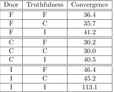
Another advantage of our Bayesian scheme is the ability to incorporate prior information to guide the algorithm. On the other hand, specifying an incorrect prior can potentially deteriorate performance instead of enhancing it. In Table 4, we provide performance results from employing an informed prior over T and D. With the correct underlying values
λ∗ =π = 0.85, we specify three types of priors: Correct∝N(µ= 0.85, σ= 0.3), Incorrect
∝ N(µ = 0.15, σ = 0.3) and Flat (all solutions equally probable), denoted C, I, and F, respectively. We can see the effect of these different priors in Table 4. In brief, having a correct prior over the doors contributes more to convergence time than having a correct prior over the truthfulness of the guards. The disadvantage of setting an incorrectly biased prior is also evident, as the flat prior performs better than any combination involving a incorrectly biased prior.
3.2 Tracking the Truthfulness of the Environment
An interesting property of TS-SPL is its ability to provide a distribution over the truth-fulness π of the environment. This can be a significant advantage because information on
π can be leveraged in various ways. As an example, information on π can be used in the case of repeated trials, where the information from previous trials can be used as a prior in subsequent trials, greatly increasing convergence speed (cf. Section 3.1). Figure 1 plots the probability of each level of noise as the TS-SPL progresses with noise probability π = 0.15 (a highly deceptive environment). As seen, TS-SPL is capable of quickly estimating π
accurately.
3.3 Stochastic Point Location
The N-Door Puzzle, as outlined in the introduction, is dependent on two variablesλ∗ and
π∗, with λ∗ specifying the door leading to freedom and π∗ the truthfulness of the guards. Since the N-Door Puzzle does not pose any spatial requirements on the placements of the doors we can generate a mapping from the N-Door Puzzle to the SPL problem by uniformly placing the doors over the unit interval.
Door Truthfulness Convergence
F F 36.4
F C 35.7
F I 41.2
C F 30.2
C C 30.0
C I 40.5
I F 46.4
I C 45.2
I I 113.1
Table 4: Convergence steps for TS-SPL solving the N-Door Puzzle with different priors: C - Correct Prior, F - Flat Prior, I - Incorrect prior. Here, λ∗ = 0.85, I ={0.15±0.01},
|T|=|D|= 101, and π= 0.85.
0.0 0.2 0.4 0.6 0.8 1.0
0.00
0.02
0.04
0.06
0.08
π
probability
it=0 (prior) it=10 it=20 it=100 it=200
actions. In the case of SPL we define regret as the (unsigned) distance between the selected point x and the optimal pointλ∗.
3.3.1 Informative SPL
We first evaluate the performance of TS-SPL and TS-SPL-INF on an informative SPL problem, in comparison with algorithms designed to handle informative environments. To the best of our knowledge this is the first time both the family of PBS based schemes and the family of SPL based schemes are compared.
The performance of the different schemes is summarized in Table 5. One significant ob-servation is the performance difference between the Learning Automata (LA) based schemes (HSSL and SHSSL) and the Bayesian schemes. It is clear that performance-wise, Bayesian schemes significantly outperform the LA based schemes. However, it should be noted that the LA based schemes require less memory and run faster than the Bayesian ones due to their simplicity.
As seen in Table 5, the distance|12−λ∗|is an important metric for how hard a particular SPL problem is to solve. This can be explained by the fact that most schemes start exploring from the center. Thus, ifλ∗is far from the center, such a scheme needs more evidence before it starts exploring the peripheral regions of the search space. This is particularly apparent for PBS-M as its performance peaks in the case where λ∗ = 0.25, even when faced with significant noise (π = 0.65).
Since PBS-M pursues the median of the probability distribution, we can say that PBS-M is conservative in its exploration. This is because it takes significant more evidence to move the point of exploration compared to TS-SPL. TS-SPL, on the other hand, has a tendency to explore too much. Indeed, as noted by Lattimore (Lattimore, 2015), using TS for exploration can lead to over-exploration when facing high variance distributions. In the low noise scenarios, however, NGBS-M is the most efficient scheme, exploring deterministically. For PT-PBS, we observe throughout all the experiments significantly worse performance than PBS-M. We thus omit the PT-PBS results for the remaining experiments, focusing on PBS-M instead.
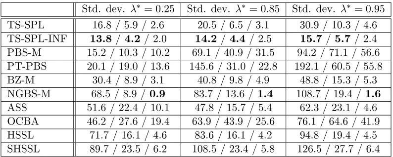
Finally, from Table 6 we observe that TS-SPL-INF exhibits the lowest standard deviation overall, and is consequentially the scheme that consistently perform closest to its expected regret for every trial. This is in sharp contrast to PBS-M who outperform TS-SPL when it comes to average regret, but is unable to do so consistently. NGBS-M also displays significant variance in high noise scenarios.
3.3.2 SPL in Deceptive Environments
Avg Regret λ∗= 0.25 Avg Regret λ∗ = 0.85 Avg Regretλ∗= 0.95
TS-SPL 29.2 / 9.8 / 5.1 36.4 / 12.9 / 6.2 57.3 / 20.3 / 10.1 TS-SPL-INF 22.2 / 7.3 / 3.7 22.5 / 7.7 / 3.8 23.9/ 8.7 / 4.3 PBS-M 9.8/ 4.0 / 2.6 32.7 / 14.2 / 8.5 52.1 / 29.6 / 16.9 PT-PBS 245.4 / 247.5 / 247.4 548.2 / 751.5 / 785.2 551.4 / 815.0 / 828.4 BZ-M 23.5 / 5.9 / 2.2 27.5 / 6.3 / 2.5 35.1 / 9.6 / 3.4 NGBS-M 36.9 /3.5 / 1.0 48.9 /4.5 /1.5 68.5 /7.1/ 2.3 ASS 45.8 / 17.0 / 6.7 30.4 / 8.9 / 3.6 38.8 / 11.7 / 3.9 OCBA 70.8 / 47.4 / 35.2 89.9 / 55.8 / 37.1 112.1 / 78.4 / 48.8 HSSL 117.3 / 23.1 / 8.2 111.7 / 16.7 / 4.8 131.5 / 19.1 / 5.3 SHSSL 152.2 / 32.6 / 11.8 151.8 / 23.5 / 6.5 175.1 / 26.1 / 7.3
Table 5: Average regret for the different schemes in an informative SPL. The result is reported in the format a/b/c, where a is the average regret for π = 0.65, b for π = 0.75, and cforπ = 0.85. The number of time steps per trial is 1000.
Std. dev. λ∗= 0.25 Std. dev. λ∗ = 0.85 Std. dev. λ∗ = 0.95
TS-SPL 16.8 / 5.9 / 2.6 20.5 / 6.5 / 3.1 30.9 / 10.3 / 4.6 TS-SPL-INF 13.8 / 4.2/ 2.0 14.2 / 4.4/ 2.5 15.7 /5.7 / 2.4 PBS-M 15.2 / 10.3 / 10.2 69.1 / 40.9 / 31.5 94.2 / 71.1 / 56.6 PT-PBS 20.1 / 19.0 / 13.6 145.6 / 31.0 / 22.8 192.1 / 60.5 / 55.8 BZ-M 30.4 / 8.9 / 3.1 40.8 / 9.8 / 4.9 48.8 / 15.3 / 5.3 NGBS-M 68.5 / 8.9 /0.9 83.7 / 13.6 / 1.4 108.7 / 19.4 /1.6 ASS 51.6 / 22.4 / 10.1 47.8 / 15.7 / 5.4 62.3 / 23.1 / 4.6 OCBA 46.2 / 27.6 / 19.4 63.9 / 43.9 / 25.6 76.1 / 64.6 / 41.9 HSSL 71.7 / 16.1 / 4.6 83.6 / 16.1 / 4.2 94.8 / 19.4 / 4.5 SHSSL 89.7 / 23.5 / 6.2 108.5 / 23.4 / 5.8 126.5 / 27.7 / 6.4
π = 0.85 π = 0.15 TS-SPL (λ∗ = 0.85) 6.2 6.2 CPL-AdS (λ∗= 0.85) 501.6 / 354.9 842.8/502.3
PBS-M (λ∗ = 0.85) 31.5 77.5 BZ-M (λ∗ = 0.85) 4.9 352.5 NGBS-M (λ∗ = 0.85) 1.4 191.2 SHSSL (λ∗ = 0.85) 6.5 6.5
Table 7: Cumulative regret for the deceptive SPL problem after N = 1000 time steps. For CPL-AdS, we report both the total accumulated regret, as well as regret obtained after the nature of the environment has been decided.
Another interesting observation is that the performance of TS-SPL is symmetric around 0.5. Further note that SHSSL fails to converge for π ∈ [0.382,0.682], as stated earlier. Hence, SHSSL is effectively operating with a 30% smaller search space for π than both TS-SPL and CPL-AdS.
After modifying PBS, NGBS and BZ to support a Bayesian model of truthfulness, we can use the same prior that we apply in TS-SPL also for these schemes, leading to PBS-M, NGBS-M and BZ-M. The effect of this enhancement to existing schemes is summarized in Table 7. As clearly seen, the query selection method for these schemes is not suited to handle deceptive environments.
3.4 Stochastic Root-Finding
The deterministic root finding problem concerns locating a root x∗ of a function g(x), defined over an interval (a, b) [i.e., findingx∗,g(x∗) = 0]. We assume thatg(x) is unknown, however, an oracle returns the value of g(x) at any point x queried. The problem is then how to determine the root x∗ using as few queries as possible. One approach to solving the deterministic root finding problem is the Bisection Method. This approach halves the search space in each iteration by continually querying the oracle using the midpoint of the remaining search space.
If the response from the oracle is noisy, we obtain the SRF problem (Pasupathy and Kim, 2011). We define the SRF problem as follows. For anyx∈(0,1), the oracle generates a sample Y(x) = g(x) +wnoise, where wnoise is a random variable with mean zero. Let S(x) denote the sign of Y(x): S(x) = sgn[Y(x)]. Notice that the noisewnoise may render
sgn[Y(x)] different from sgn[g(x)]. Thus, with noisy feedback, the Bisection Method may discard the wrong half of the search space. The challenge is then how to select a sequence of queries x1, x2, . . . , xn to gather information on x∗, so that the final query xn is close to
x∗,|xn−x∗|< , despite the noise (Waeber et al., 2011). Note that in the SRF problems we
investigate here,S(x) returns sgn[g(x)] with probability π and−sgn[g(x)] with probability 1−π.
Implementation-wise SA methods3 extend or modify the iterative Newton-Raphson algorithm to handle noise:
xn+1 =xn−anYn(xn)
where{an}is a sequence of step lengths that decreases as nincreases.
Approaches for applying SA to the SRF problem has been extensively studied in the literature. It is outside the scope of this article to give a full literature review, however, interested readers are referred to surveys in recent studies (Lai, 2003; Asmussen and Glynn, 2007; Pasupathy and Kim, 2011). As there exists a myriad of different SA approaches, we have selected one of the more fundamental ones to form a basis for contrasting the different schemes.
Note that the SA approach we use here requires that g(x) is monotonic. This can be explained as follows. The main difference between SRF and SPL is that, unlike SPL, the SRF oracle does not directly provide feedback on the direction of the root x∗ from the query locationx. However, for monotonicg(x), one can obtain this direction from the sign of Y(x), S(x) ∈ {−1,1} and from the derivative g0(x) of g(x). If g(x) is increasing and
S(x) = 1, then the direction derived from the oracle is ”to the left ofx” [and ”to the right” ifS(x) =−1]. Conversely, if g(x) is decreasing and S(x) = 1, then the direction obtained is ”to the right ofx” [and ”to the left” if S(x) =−1].
TS-SPL, on the other hand, does not need to know the derivative of g(x). Indeed,
g(x) does not even need to be monotonic. Instead, TS-SPL merely requires an arbitrary mapping of the sign S(x) to a direction. One could, for instance, define positive to mean ”left”, S(x) = 1 ⇒ left, and negative to mean ”right”, S(x) = −1 ⇒ right. If it turns out that the opposite is the case, TS-SPL will recognize that the feedback is deceptive and still solve the problem. An informative scheme, on the other hand, will be misled in such a deceptive environment.
Informative SPL schemes can also be used for SRF problems. However, then we need an initial sampling step that decides the nature of the functiong(x). Learning whether the functiong(x) starts above zero and falls below zero, or vice versa, can be done by repeatedly querying a single point on the edge of the interval (0,1), obtaining multiple samples from either S(x). In brief, by estimating E[S(x)], we can decide the nature of g(x). To gain insight into how many repeated samples are sufficient for estimatingE[S(x)] accurately, we employ the two sided Hoeffding’s inequality P(|X¯ −E[ ¯X]| ≥ δ) ≤2e−2nδ2. Here, ¯X is the average ofnqueries at xand δ is a value such that |π−1
2| ≥δ. Setting the rhs. equal to p and solving forn, we obtainn≥ −log(2δp/22). Plugging in forδ= 0.05 andp= 0.99 we obtain dne= 62. Thus we are 99% sure of our estimate ofS(x), given that |π−0.5| ≥0.05.
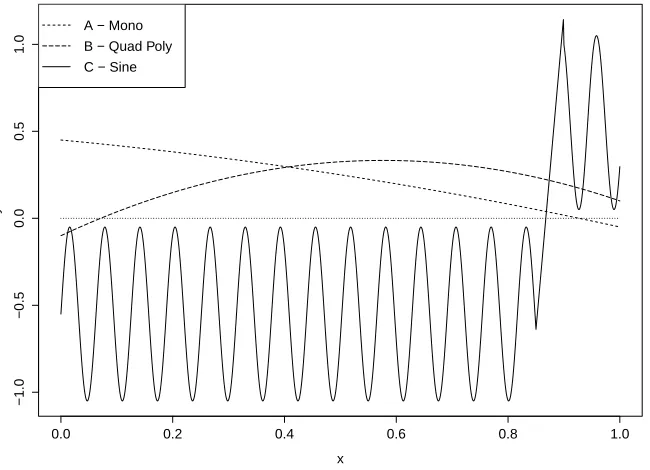
The functions that we use to measure performance and compare schemes are illustrated in Figure 2. From Table 8, 9 and 10 it is clear that TS-SPL is the most efficient root solver among state-of-the-art schemes. We believe this largely comes from the fact that it simultaneously learns the nature of the oracle (informative or deceptive), as well as trying to locate the root x∗. In addition, there is the risk that the sampling procedure that the other schemes apply to determine which direction g(x) is increasing may conclude with the wrong answer. If this happens, none of the schemes depending on the sampling will
0.0 0.2 0.4 0.6 0.8 1.0
−1.0
−0.5
0.0
0.5
1.0
x
y
A − Mono B − Quad Poly C − Sine
Figure 2: The three functions A, B and C for benchmarking stochastic root finding schemes.
Func A Avg Regret. π = 0.65 Avg Regret. π = 0.75 Avg Regretπ = 0.85
TS-SPL 46.0 17.1 8.6
TS-SPL-INF 55.2 (24.3) 39.1 ( 8.1 ) 35.0 ( 4.1 ) PBS-M 55.1 (24.2) 40.3 ( 9.3 ) 35.2 ( 4.2 ) NGBS-M 53.4 (22.4) 35.3 ( 4.3 ) 32.9 ( 1.9 ) BZ-M 63.8 (32.8) 39.9 ( 8.9 ) 33.8 ( 2.8 )
SA 32.4 14.8 5.4
ASS 80.4 (49.4) 38.7 ( 7.7 ) 33.5 ( 2.5 ) HSSL 60.4 (29.4) 45.5 ( 14.6 ) 35.8 ( 4.8 )
SHSSL 62.8 20.2 6.7
CPL-AdS 162.1 (107.9) 146.3 (97.4) 135.3 (90.1)
Func B Avg Regret. π = 0.65 Avg Regret. π = 0.75 Avg Regretπ = 0.85
TS-SPL 47.1 17.8 8.5
TS-SPL-INF 53.8 ( 22.9 ) 39.5 ( 8.5 ) 35.1 ( 4.1 ) PBS-M 41.1 ( 10.2 ) 35.3 ( 4.31 ) 33.3 ( 2.3 ) SGBS-M 50.6 ( 19.7 ) 35.7 ( 4.7 ) 33.0 ( 2.0 ) BZ-M 60.3 ( 29.4 ) 39.6 ( 8.7 ) 33.6 ( 2.6 )
SA 175.1 204.5 223.3
ASS 81.6 ( 50.6 ) 39.5 ( 8.7 ) 40.2 ( 9.0 ) HSSL 85.3 ( 54.4 ) 50.6 ( 19.6 ) 39.0 ( 8.0 )
SHSSL 75.4 30.8 12.7
CPL-AdS 117.9 (109.3) 116.7 (107.1) 144.9 (96.5)
Table 9: Average residuals for the different schemes when finding the root of the quadric function B under various noise levels. The root isx∗ = 0.9270. The results are given in the format ”average residuals (average residuals after sampling)” for each scheme. For CPL-AdS the sampling period is the estimation period (epoch 0) as defined by the scheme. The number of iterations per trial is 250.
Func C Avg Regret. π = 0.65 Avg Regret. π = 0.75 Avg Regretπ = 0.85
TS-SPL 36.9 13.7 6.4
TS-SPL-INF 52.8 ( 21.9 ) 38.8 ( 7.8 ) 34.9 ( 3.9 ) PBS-M 49.6 ( 18.7 ) 39.2 ( 8.3 ) 34.3 ( 3.3 ) SGBS-M 47.2 ( 16.2 ) 34.6 ( 3.6 ) 32.5 ( 1.6 ) BZ-M 58.8 ( 27.9 ) 38.4 ( 7.4 ) 33.7 ( 2.7 )
SA 149.0 178.0 185.0
ASS 54.3 ( 23.4 ) 39 ( 8.0 ) 33.5 ( 2.5 ) HSSL 75.2 ( 44.3 ) 44.3 ( 13.4 ) 35.6 ( 4.6 )
SHSSL 56.5 18.4 6.4
CPL-AdS 153.0 (101.6) 156.2 (103.7) 165.0 (109.6)
converge towards the rootx∗. A perhaps even stronger advantage of TS-SPL is that it can be applied to a wide range of functions without regards to the presence of local extrema. SA, on the other, only performs well for monotonic functions as exemplified in Table 8.
4. Conclusions and Further Work
In this paper, we investigated a novel reinforcement learning problem derived from the so-called ”N-Door Puzzle”. This puzzle has the fascinating property that it involves stochastic compulsive liars. Feedback is erroneous on average, systematically misleading the decision maker. This renders traditional reinforcement learning (RL) based approaches ineffective due to their dependency on ”on average” correct feedback.
To solve the problem of deceptive feedback, we recast the problem as a challenging variant of the multi-armed bandit problem, referred to as the Stochastic Point Location (SPL) problem. In SPL, the decision maker is only told whether the optimal point on a line lies to the “left” or to the “right” of a current guess, with the feedback being erroneous with probability 1−π. Solving this problem opens up for optimization in continuous action spaces with bothinformativeand deceptive feedback.
Our solution to the above problem, introduced in the present paper, is based on a novel Bayesian representation of the solution space that is both compact and scalable. This model simultaneously captures both the location of the optimal point, as well as the probability of receiving correct feedbackπ. We further introduced an accompanying Thompson Sampling (TS) guided Stochastic Point Location (TS-SPL) scheme for balancing exploration against exploitation. By learningπ, TS-SPL supports deceptive environments that are lying about the direction of the optimal point.
We used TS-SPL to solve the Stochastic Point Location (SPL) problem and outper-formed all of the Learning Automata driven methods. However, by enhancing the Soft Generalized Binary Search (SGBS) scheme with our Bayesian representation of the solution space, SGBS was able to outperform TS-SPL under informative feedback. For deceptive SPL problems, TS-SPL outperformed all of the existing state-of-art schemes by several orders of magnitude, even when the latter schemes were supported by our Bayesian model. We also applied TS-SPL to the Stochastic Root Finding (SRF) problem. We further demonstrated that SRF can be seen as a deceptive problem, allowing TS-SPL to outperform existing dedicated state-of-art SRF schemes by an order of magnitude. Thus, TS-SPL can be considered state-of-the-art for both deceptive SPL and for SRF, while yielding comparable results to the top performing schemes in the case of informative SPLs.
Despite the above performance gains, TS-SPL is based on Thompson Sampling, which is known to have a tendency to over-explore high variance reward distributions (Lattimore, 2015). In future work, it is therefore interesting to investigate mechanisms that eliminate or reduce this tendency, to further increase convergence speed.
References
Shipra Agrawal and Navin Goyal. Analysis of thompson sampling for the multi-armed bandit problem. In Conference on Learning Theory, pages 39–1, 2012.
Shipra Agrawal and Navin Goyal. Further optimal regret bounds for thompson sampling. In Proceedings of the 16th Conference on Artificial Intelligence and Statistics, pages 99–107, 2013a.
Shipra Agrawal and Navin Goyal. Thompson sampling for contextual bandits with linear payoffs. InProceedings of the 30th International Conference on Machine Learning (ICML-13), pages 127–135, 2013b.
Soren Asmussen and Peter W Glynn. Stochastic simulation: Algorithms and Analysis, volume 57. Springer Science & Business Media, 2007.
Onur Atan, Cem Tekin, and Mihaela van der Schaar. Global multi-armed bandits with h¨older continuity. InProceedings of the 18th International Conference on Artificial Intel-ligence and Statistics, pages 28–36, 2015.
Jean-Yves Audibert and S´ebastien Bubeck. Best arm identification in multi-armed bandits. In Conference on Learning Theory, pages 13–p, 2010.
S´ebastien Bubeck and Nicolo Cesa-Bianchi. Regret analysis of stochastic and nonstochastic multi-armed bandit problems. Machine Learning, 5(1):1–122, 2012.
Marat Valievich Burnashev and Kamil’Shamil’evich Zigangirov. An interval estimation problem for controlled observations. Problemy Peredachi Informatsii, 10(3):51–61, 1974.
Rui M Castro and Robert D Nowak. Upper and lower error bounds for active learning. In In Proceedings of the 44th Conference on Communication, Control and Computing, volume 2, page 1, 2006.
Olivier Chapelle and Lihong Li. An empirical evaluation of thompson sampling. In Pro-ceedings of the Advances in Neural Information Processing Systems 24, pages 2249–2257. Curran Associates, Inc., 2011.
Huifen Chen and Bruce W Schmeiser. Stochastic root finding via retrospective approxima-tion. IIE Transactions, 33(3):259–275, 2001.
Shi Dong and Benjamin Van Roy. An information-theoretic analysis for thompson sampling with many actions. In Proceedings of the Advances in Neural Information Processing Systems 31, pages 4157–4165, 2018.
Eyal Even-Dar, Shie Mannor, and Yishay Mansour. Action elimination and stopping con-ditions for the multi-armed bandit and reinforcement learning problems. Journal of Machine Learning Research, 7(Jun):1079–1105, 2006.
Victor Gabillon, Mohammad Ghavamzadeh, Alessandro Lazaric, and S´ebastien Bubeck. Multi-bandit best arm identification. In Proceedings of the Advances in Neural Informa-tion Processing Systems 24, pages 2222–2230, 2011.
Sondre Glimsdal and Ole-Christoffer Granmo. Gaussian process based optimistic knap-sack sampling with applications to stochastic resource allocation. In Proceedings of the 24th Midwest Artificial Intelligence and Cognitive Science Conference 2013, pages 43–50. CEUR Workshop Proceedings, 2013.
Ole-Christoffer Granmo. Solving two-armed bernoulli bandit problems using a bayesian learning automaton. International Journal of Intelligent Computing and Cybernetics, 3 (2):207–234, 2010.
Ole-Christoffer Granmo and Sondre Glimsdal. Accelerated bayesian learning for decen-tralized two-armed bandit based decision making with applications to the goore game. Applied intelligence, 38(4):479–488, 2013.
Ole-Christoffer Granmo, B John Oommen, Svein Arild Myrer, and Morten Goodwin Olsen. Learning Automata-based Solutions to the Nonlinear Fractional Knapsack Problem with Applications to Optimal Resource Allocation. IEEE Transactions on Systems, Man, and Cybernetics, Part B, 37(1):166–175, 2007.
Michael Horstein. Sequential transmission using noiseless feedback. IEEE Transactions on Information Theory, 9(3):136–143, 1963.
Laurent Hyafil and Ronald L Rivest. Constructing optimal binary decision trees is np-complete. Information Processing Letters, 5(1):15–17, 1976.
Kevin Jamieson, Matthew Malloy, Robert Nowak, and S´ebastien Bubeck. lil’ucb: An opti-mal exploration algorithm for multi-armed bandits. In Conference on Learning Theory, volume 35, pages 423–439, 2014.
Y Yu Jia and Shie Mannor. Unimodal bandits. In International Conference on Machine Learning, pages 41–48, 2011.
Lei Jiao, Xuan Zhang, B. John Oommen, and Ole-Christoffer Granmo. Optimizing channel selection for cognitive radio networks using a distributed bayesian learning automata-based approach. Applied Intelligence, 44(2):307–321, 2016. ISSN 1573-7497.
Zohar Shay Karnin, Tomer Koren, and Oren Somekh. Almost optimal exploration in multi-armed bandits. International Conference on Machine Learning, 28:1238–1246, 2013.
Jack Kiefer and Jacob Wolfowitz. Stochastic estimation of the maximum of a regression function. The Annals of Mathematical Statistics, 23(3):462–466, 1952.
HJ Kushner and G Yin. Stochastic approximation algorithms for parallel and distributed processing.Stochastics: An International Journal of Probability and Stochastic Processes, 22(3-4):219–250, 1987.
Tor Lattimore. Optimally confident ucb: Improved regret for finite-armed bandits. arXiv preprint arXiv:1507.07880, 2015.
Robert Nowak. Generalized binary search. In Communication, Control, and Computing, 2008 46th Annual Allerton Conference on, pages 568–574. IEEE, 2008.
Robert D Nowak. The geometry of generalized binary search. Information Theory, IEEE Transactions on, 57(12):7893–7906, 2011.
B John Oommen. Stochastic Searching on the Line and its Applications to Parameter Learn-ing in Nonlinear Optimization. IEEE Transactions on Systems, Man, and Cybernetics, Part B, 27(4):733–739, 1997.
B John Oommen, Govindachari Raghunath, and Benjamin Kuipers. On how to learn from a stochastic teacher or a stochastic compulsive liar of unknown identity. In AI 2003: Advances in Artificial Intelligence, pages 24–40. Springer, 2003.
B John Oommen, Sudip Misra, and Ole-Christoffer Granmo. Routing bandwidth-guaranteed paths in mpls traffic engineering: A multiple race track learning approach. IEEE Transactions on Computers, 56(7):959–976, 2007.
B John Oommen, Ole-Christoffer Granmo, and Zuoyuan Liang. A novel multidimensional scaling technique for mapping word-of-mouth discussions. In Opportunities and Chal-lenges for Next-Generation Applied Intelligence, pages 317–322. Springer, 2009.
Stephen Pallone, Peter I Frazier, and Shane G Henderson. Multisection: Parallelized bisec-tion. In Simulation Conference, Winter, pages 3773–3784. IEEE, 2014.
Raghu Pasupathy and Sujin Kim. The stochastic root-finding problem: Overview, solutions, and open questions. ACM Transactions on Modeling and Computer Simulation, 21(3): 19, 2011.
Raghu Pasupathy and Bruce W Schmeiser. Root finding via darts – dynamic adaptive ran-dom target shooting. In Simulation Conference (WSC), Proceedings of the 2010 Winter, pages 1255–1262. IEEE, 2010.
Andrzej Pelc. Searching games with errors – fifty years of coping with liars. Theoretical Computer Science, 270(1):71–109, 2002.
Herbert Robbins and Sutton Monro. A stochastic approximation method. The annals of mathematical statistics, pages 400–407, 1951.
Aarti Singh, Robert Nowak, and Parmesh Ramanathan. Active learning for adaptive mobile sensing networks. In In Proceedings of the 5th international conference on Information processing in sensor networks, pages 60–68. ACM, 2006.
Tongtong Tao, Hao Ge, Guixian Cai, and Shenghong Li. Adaptive step searching for solving stochastic point location problem. In Intelligent Computing Theories, pages 192–198. Springer, 2013.
William R Thompson. On the likelihood that one unknown probability exceeds another in view of the evidence of two samples. Biometrika, 25(3/4):285–294, 1933.
David Tolpin and Frank Wood. Maximum a posteriori estimation by search in probabilistic programs. In Proceedings of the 8th Annual Symposium on Combinatorial Search, 2015.
Rolf Waeber, Peter Frazier, and Shane G Henderson. A bayesian approach to stochastic root finding. InProceedings of the 2011 Winter Simulation Conference, pages 4033–4045. IEEE, 2011.
Rolf Waeber, Peter I Frazier, and Shane G Henderson. Bisection search with noisy responses. SIAM Journal on Control and Optimization, 51(3):2261–2279, 2013.
Anis Yazidi, Ole-Christoffer Granmo, B John Oommen, and Morten Goodwin. A hierar-chical learning scheme for solving the stochastic point location problem. In Advanced Research in Applied Artificial Intelligence, pages 774–783. Springer, 2012a.
Anis Yazidi, B John Oommen, and Ole-Christoffer Granmo. A novel stochastic discretized weak estimator operating in non-stationary environments. In Proceedings of the Inter-national Conference on Computing, Networking and Communications, pages 364–370. IEEE, 2012b.
Junqi Zhang, Liang Zhang, and Mengchu Zhou. Solving stationary and stochastic point location problem with optimal computing budget allocation. In Proceedings of the 2015 IEEE International Conference on Systems, Man, and Cybernetics, pages 145–150, Oct 2015. doi: 10.1109/SMC.2015.38.