A Note on Quickly Sampling a Sparse Matrix with Low Rank Expectation

A Note on Quickly Sampling a Sparse Matrix with Low Rank

Expectation

Karl Rohe [email protected]

Statistics Department

University of Wisconsin-Madison Madison, WI 53706, USA

Jun Tao [email protected]

School of Mathematical Sciences Peking University

Beijing, 100871, China

Xintian Han [email protected]

Yuanpei College Peking University Beijing, 100871, China

Norbert Binkiewicz [email protected]

Statistics Department

University of Wisconsin-Madison Madison, WI 53706, USA

Editor:Inderjit Dhillon

Abstract

Given matricesX,Y∈Rn×K_andS∈RK×K_{with positive elements, this paper proposes an algorithm}

fastRGto sample a sparse matrixAwith low rank expectationE(A) =X SYT and independent Pois-son elements. This allows for quickly sampling from a broad class of stochastic blockmodel graphs (degree-corrected, mixed membership, overlapping) all of which are specific parameterizations of the generalized random product graph model defined in Section 2.2. The basic idea offastRGis to first sample the number of edgesmand then sample each edge. The key insight is that because of the the low rank expectation, it is easy to sample individual edges. The naive “element-wise” algo-rithm requiresO(n2)operations to generate then×nadjacency matrixA. In sparse graphs, where

m=O(n), ignoring log terms,fastRGruns in timeO(n). An implementation inRis available on github. A computational experiment in Section 2.4 simulates graphs up ton=10,000,000 nodes withm=100,000,000 edges. For example, on a graph withn=500,000 andm=5,000,000, fastRGruns in less than one second on a 3.5 GHz Intel i5.

Keywords: Random Dot Product Graph, Edge exchangeable, Simulation

1. Introduction

The random dot product graph (RDPG) model serves as a test bed for various types of clustering and statistical inference algorithms. This model generalizes the Stochastic Blockmodel (SBM), the Overlapping SBM, the Mixed Membership SBM, and the Degree-Corrected SBM (Holland et al., 1983; Latouche and Ambroise, 2011; Airoldi et al., 2008; Karrer and Newman, 2011). Under the

c

RDPG, each nodeihas a (latent) node featurexi∈RK and the probability that nodeiand jshare

an edge is parameterized byhxi,xji(Young and Scheinerman, 2007).

While many network analysis algorithms only requireO(m)operations, wheremis the number of edges in the graph, sampling RDPGs with the naive “element-wise” algorithm takesO(n2) op-erations, wherenis the number of nodes. In particular, sparse eigensolvers compute the leadingk

eigenvectors of such graphs inO(km)operations (e.g. in ARPACK Lehoucq et al. 1995). As such, sampling an RDPG is a computational bottleneck in simulations to examine many network analysis algorithms.

The organization of this paper is as follows. Section 2 givesfastRG. Section 2.1 relatesfastRG to xlr, a new class of edge-exchangeable random graphs with low-rank expectation. Section 2.2 presents a generalization of the random dot product graph. Theorem 4 shows thatfastRGsamples Poisson-edge graphs from this model. Then, Theorem 7 in Section 2.3 shows how fastRGcan be used to approximate a certain class of Bernoulli-edge graphs. Section 2.4 describes our imple-mentation of fastRG(available at https://github.com/karlrohe/fastRG) and assesses the empirical run time of the algorithm.

1.1. Notation

LetG= (V,E)be a graph with the node setV={1, . . . ,n}and the edge setEcontains edge(i,j)if nodeiis connected to node j. In a directed graph, each edge is an ordered pair of nodes while in an undirected graph, each edge is an unordered pair of nodes. A multi-edge graph allows for repeated edges. In any graph, a self-loop is an edge that connects a node to itself. Let the adjacency matrix

A∈Rn×n_{contain the number of edges fromito jin elementA}

i j. For column vectorsx∈Ra,z∈Rb

andS∈_Ra×b_{, definehx,zi}

S=xTSz; this function is not necessarily a proper inner product because

it does not require thatSis non-negative definite. We use standard big-Oand little-onotations, i.e. for sequencexn,yn;xn=o(yn)when ynis nonzero implies limn→∞xn/yn=0;xn=O(yn)implies

there exists a positive real numberMand an integerNsuch that|xn| ≤M|yn|, ∀n≥N.

2. fastRG

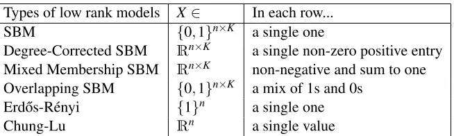
fastRGis motivated by the wide variety of low rank graph models that specify the expectation of the adjacency matrix asE(A) =X SXT for some matrix (or vector)X and some matrix (or value)S.

Types of low rank models X∈ In each row... SBM {0,1}n×K _{a single one}

Degree-Corrected SBM Rn×K a single non-zero positive entry Mixed Membership SBM Rn×K non-negative and sum to one Overlapping SBM {0,1}n×K _{a mix of 1s and 0s}

Erd˝os-R´enyi {1}n _{a single one}

Chung-Lu Rn a single value

Given X ∈_Rn×Kx_{, Y} ∈_Rd×Ky _{and S}∈_RKx×Ky_{, fastRG samples a random graph. Define A}

as then×d matrix whereAi j counts the number of times edge(I,J)was sampled by fastRG. In

expectation A is X SYT. Importantly, fastRGrequires that the elements of X,Y,and S are non-negative. This condition holds for all of the low rank models in the above table. Each of those models setY =X and enforce different restrictions on the matrixX.

As stated below,fastRGsamples a (i) directed graph with (ii) multiple edges and (iii) self-loops. After sampling, these properties can be modified to create a simple graph (undirected, no repeated edges, and no self-loops); see Remarks 5 and 6 in Section 2.2 and Theorem 7 in Section 2.3.

Algorithm 1fastRG(X,S,Y)

Require: X∈_Rn×Kx_,S∈RKx×Ky_{, andY∈R}d×Ky_{with all matrices containing non-negative entries.}

Compute diagonal matrixCX ∈RKx×Kx withCX=diag(∑iXi1, . . . , ∑iXiKx).

Compute diagonal matrixCY∈RKy×Ky withCY =diag(∑iYi1, . . . , ∑iYiKy).

Define ˜X=XC_X−1, ˜S=CXSCY, and ˜Y =YCY−1.

Sample the number of edgesm∼Poisson(∑u,vS˜uv).

for`=1 :mdo

SampleU∈ {1, . . . , Kx},V ∈ {1, . . . , Ky}withP(U=u,V=v)∝S˜uv.

SampleI∈ {1, . . . , n}withP(I=i) =X˜iU.

SampleJ∈ {1, . . . , d}withP(J= j) =Y˜jV.

Add edge(I,J)to the graph, allowing for multiple edges(I,J).

end for

An implementation in Ris available at https://github.com/karlrohe/fastRG. As dis-cussed in Section 2.4, in order to make the algorithm more efficient, the implementation is slightly different from the statement of the algorithm above.

There are two model classes that can help to interpret the graphs generated from fastRGand those model classes are explored in the next two subsections. Throughout all of the discussion, the key fact that is exploited byfastRGis given in the next Theorem.

Theorem 1 Suppose that X∈_Rn×Kx_{, Y}∈_Rd×Ky_{and S}∈_RKx×Ky _{all contain non-negative entries.}

Define xi∈RKx as the ith row of X . Define yj∈RKy as the jth row of Y . Let(I,J)be a single edge

sampled inside the for loop infastRG(X,S,Y), then

P((I,J) = (i,j))∝hxi,yjiS.

Proof

P (I,J) = (i,j) =

_∑

u,v

P((I,J) = (i,j)|(U,V) = (u,v))P((U,V) = (u,v)))

= ∑u,v

˜

XiuY˜jvS˜uv

∑u,vS˜u,v

=∑u,vXiuYjvSuv

∑u,vS˜u,v

= x

T i Syj

2.1.fastRGsamples from xlr: a class of edge-exchangeable random graphs

There has been recent interest in edge exchangeable graph models with blockmodel structure (e.g. Crane and Dempsey 2016; Cai et al. 2016; Herlau et al. 2016; Todeschini and Caron 2016). To characterize a broad class of such models, we propose xlr. For notational simplicity, the rest of the paper will suppose thatY=X∈_Rn×K_and

fastRG(X,S) =fastRG(X,S,X).

Definition 2 [xlr] An xlr graph on n nodes and K dimensions is generated as follows,

1. Sample(X,S)∈_Rn×K_×

RK×Kfrom some distribution and define xias the ith row of X .

2. Initialize the graph to be empty.

3. Add independent edges e₁,e₂, . . .to the graph, where

P(e`= (i,j)) =

hxi,xjiS

∑a,bhxa,xbiS

.

From Theorem 1,fastRGsamples the edges in xlr.

An xlr graph is both (i) edge-exchangeable as defined by Crane and Dempsey (2016) and (ii) conditional onX andS, its expected adjacency matrix is low rank. By samplingX to satisfy one set of restrictions specified in Table 1, xlr provides a way to sample edge exchangeable blockmodels. xlr stands foredge-exchangeable and low rankbecause it characterizes all edge-exchangeable and low rank random graph models on a finite number of nodes. In particular, by Theorem 4.2 in Crane and Dempsey (2016) if a random undirected graph with an infinite number of edges is edge exchangeable, then the edges are drawn iid from some randomly chosen distribution on edges f. Moreover, letBbe the adjacency matrix of a single edge drawn from f. Under the assumption that

E(B|f)is rankK, there exist matricesX∈_Rn×K_andS∈

RK×Kthat are a function of fand give the eigendecompositionE(B|f) =X SXT_{. This implies that}

P(e1= (i,j)|f)∝hxi,xjiS, wherexi is the

ith row ofX.

2.2.fastRGsamples from a generalization of the RDPG

Under the RDPG as described in Young and Scheinerman (2007), the expectation of the adjacency matrix isX XT for some matrixX∈_Rn×K_{. This implies that the expected adjacency matrix is always}

non-negative definite (i.e. its eigenvalues are non-negative). However, some parameterizations of the SBM (and other blockmodels) lead to an expected adjacency matrix with negative eigenvalues (i.e. it is not non-negative definite); for example, if the off-diagonal elements ofSare larger than the diagonal elements, thenX SXT could have negative eigenvalues. Moreover, even if the elements of

XandSare positive, as is the case for the low rank models in Table 1 and as is required forfastRG, it is still possible forX SXT to have negative eigenvalues. By modifying the RDPG to incorporate a matrixS, the model class below incorporates all types of blockmodels.

Definition 3 [Generalized Random Product Graph (gRPG) model] For n nodes in K dimensions, the gRPG is parameterized by X∈_Rn×K _{and S∈R}K×K_{, where each node i is assigned the ith row}

of X , xi= (Xi1, . . . , XiK)T ∈RK. For i,j∈V , define

λi j=hxi,xjiS= K

∑

k K

∑

l

Under the gRPG, the adjacency matrix A∈_Rn×n_{contains independent elements and the distribution}

of Ai j (i.e. the number of edge from i to j) is fully parameterized by f(λi j), where f is some mean

function.

Below, we will use the fact that the gRPG only requires that the λi js specify the distribution of

Ai j, allowing for Ai j to be non-binary (as in multi-graphs and weighted graphs) or to have edge

probabilities which are a function ofλi j.

Theorem 4 For X ∈_Rn×K _{and S∈R}K×K_{, each with non-negative elements, ifA is the adjacency˜}

matrix of a graph sampled withfastRG(X,S), thenA is a Poisson gRPG with˜ A˜i j∼Poisson(hxi,xjiS).

The proof is contained in the appendix.

Remark 5 (Simulating an undirected graph) As defined, both the gRPG model andfastRG gen-erate directed graphs. An “undirected gRPG” should add a constraint to Definition 3 that Ai j=Aji

for all i,j. To sample such a graph with fastRG, input S/2 instead of S, then after sampling a directed graph withfastRG, symmetrize each edge by removing its direction (this doubles the prob-ability of an edge, hence the need to input S/2). Theorem 4 can be easily extended to show this is an undirected gRPG.

Remark 6 (Simulating a graph without self-loops) As defined, both the gRPG model andfastRG

generate graphs with self-loops. A “gRPG without self-loops” should add a constraint to Definition 3 that Aii=0for all i. A graph fromfastRGcan be converted to a gRPG without self-loops by

sim-ply (1) sampling m∼Poisson(∑u,vS˜uv−∑ihxi,xiiS)and (2) resampling any edge that is a self-loop.

The proof of Theorem 4 can be extended to show that this is equivalent.

2.3. Approximate Bernoulli-edges

To create a simple graph withfastRG(i.e. no multiple edges, no self-loops, and undirected), first sample a graph withfastRG. Then, perform the modifications described in Remarks 5 and 6. Then, keep an edge between iand j if there is at least one edge in the multiple edge graph; define the threshold function,t(Ai j) =1(Ai j >0), wheret(A)applies element-wise.

If ˜A is a Poisson gRPG, then t(A˜) is a Bernoulli gRPG with mean function f(λi j) = 1−

exp(−λi j). LetBbe distributed as Bernoulli gRPG(X,S) with identity mean function,

Bi j ∼Bernoulli(λi j).

Theorem 7 shows that in the sparse setting, there is a coupling betweent(A˜)andBsuch thatt(A˜)is approximately equal toB. The theorem is asymptotic inn; a superscript ofnis suppressed on ˜A,B

andλ.

Theorem 7 LetA be a Poisson gRPG and let B be a Bernoulli gRPG using the same set of˜ λi js,

withA˜i j∼Poisson(λi j)and Bi j∼Bernoulli(λi j). Let t(·)be the thresholding function forA.˜

Let αn be a sequence. If λi j =O(αn/n)for all i,j and there exists some constant c>0and

N>0such that∑i jλi j >cαnn for all n>N, then there exists a coupling between t(A˜)and B such

that

Ekt(A˜)−Bk2

F

EkBk2

F

For example, in the sparse graph setting whereλi j=O(1/n)and∑i jλi j=O(n),αn=1. Under

this setting and the coupling defined in the proof, all of theO(n) edges int(A˜)are contained inB

andBhas an extraO(1)more edges thant(A˜).

The conditionαn=o(n)implies that all edge probabilities decay. If one is interested in models

where someλi j’s are constant (e.g. certain models with heavy tailed degree distributions), then there

are three possible paths forward.

1. Segment the pairs i,j into two sets (large and smallλi j’s) and use two different sampling

techniques on each set.

2. UsefastRGas a proposal distribution for rejection sampling (if for someε >0,λi j<1−ε

for alli,j, then rejection sampling would still beO(m)operations).

3. UsefastRGand expect edge attenuation (no greater than 37%) for high probability edges.

Regarding the third point, consider the coupling in the proof of Theorem 7 without any condition onλi j. The coupling ensures that every edge int(A˜)is also contained inB. Conversely, conditioned

on edgei,jappearing inB, then the probability that this edge is included int(A˜) is a greater than 1−exp(−λi j)≥1−exp(−1)> .63.

2.4. Implementation offastRG

Code at https://github.com/karlrohe/fastRG gives an implementation offastRGin R. It also provides wrappers that simulate the SBM, Degree-Corrected SBM, Overlapping SBM, and Mixed Membership SBM. The code for these models first generates the appropriate X and then callsfastRG. In order to help control the edge density of the graph,fastRGand its wrappers can be given an additional argument avgDeg. If avgDeg is given, then the matrixSis scaled so thatfastRG simulates a graph with expected average degree equal to avgDeg. Without this, parameterizations can easily produce very dense graphs.

To accelerate the running time of fastRG, the implementation is slightly different than the statement of the algorithm above. The difference can be thought of as sampling all of the (U,V)

pairs before sampling any of the Is or Js. In particular, the implementation samplesϖ ∈RK×K

as multinomial(m,S˜/∑u,vS˜uv). Then, for eachu∈ {1, . . .K}, it samples∑vϖu,v-manyIs from the

distribution ˜X·u. Similarly, for eachv∈ {1, . . .K}, it samples∑uϖu,v-manyJs from the distribution

˜

X·v. Finally, the indexes are appropriately arranged so that there areϖu,v-many edges(I,J)where

I ∼X·u andJ∼X·v. Recall that the statement of fastRGabove allows for X andY, where those

matrices can have different numbers of rows and/or columns; the implementation also allows for this.

Under the SBM, it is possible to use fastRG to sample from the Bernoulli gRPG with the

identitymean function instead of the mean function 1−exp(−hxi,xjiS)that is created by the

thresh-olding functiont from Section 2.3. The wrapper for the SBM does this by first transforming each element ofSas−ln(1−Si j)and then callingfastRG. The others models are not amenable to this

3. Experiments

3.1. Running time offastRGon large and sparse graphs

To examine the running time offastRG, we simulated a range of different values ofn andE(m), whereE(m)is the expected number of edges. In all simulationsX=YandK=5. The elements ofX

are independentPoisson(1)random variables and the elements ofSare independentU ni f orm[0,1]

random variables. To specifyE(m), the parameter avgDeg is set toE(m)/n. The values ofnrange from 10,000 to 10,000,000 and the values ofE(m)range from 100,000 to 100,000,000. The graph was taken to be directed, with self-loops and multiple edges. Moreover, the reported times are only to generate the edge list of the random graph; the edge list is not converted into a sparse adjacency matrix, which in some experiments would have more than doubled the running time. Each pair of

nandE(m)is simulated one time; deviations around the trend lines indicate the variability in run time.

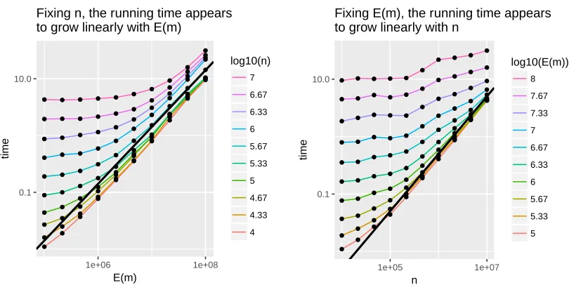
In Figure 1, the vertical axes present the running time inRon a Retina 5K iMac, 27-inch, Late 2014 with 3.5 GHz Intel i5 and 8GB of 1600 MHz DDR3 memory. In the left panel of Figure 1, each line corresponds to a single value ofn andE(m) increases along the horizontal axis. In the right panel of Figure 1, each line corresponds to a single value ofE(m)andnincreases along the horizontal axis. All axes are on thelog₁₀ scale. The solid black line has a slope of 1. Because the data aligns with this black line, this suggests thatfastRGruns in linear time.

The computational bottleneck is sampling the Is and Js. The implementation uses Walker’s Alias Method (Walker, 1977) (via sample in R). To take m samples from a distribution over n

elements, Walker’s Alias Method requires O(m+ln(n)n) operations (Vose, 1991). However, the log dependence is not clearly evident in the right plot of Figure 1; perhaps it would be visible for larger values ofn.

3.2. Comparison to a previous technique

Previously, Hagberg and Lemons (2015) studied a fast technique to generate sparse random kernel graphs. Under the random kernel graph model, nodesiand jconnect with probabilityκ(i/n,j/n), where the function κ is non-negative, bounded, symmetric, measurable, and almost surely

con-tinuous. This model class includes the SBM and the Degree-Corrected SBM. It is difficult to see how a more general low rank model could be parameterized as a random kernel graph with an al-most surely continuousκ. For example, we suspect that Mixed Membership SBMs could not be

parameterized as such.

The algorithm proposed in Hagberg and Lemons (2015) is fast when it is fast to compute (i) the integralF(y,a,b) =Rb

aκ(x,y)dxand (ii) its roots, that is for anyy,a,r, solve forF(y,a,b) =r.

Their software, which we will refer to as f ast-κis in python and generates a NetworkX graph.

For a simple benchmark to compare the running times offastRGand f ast-κ, Figure 2 repeats

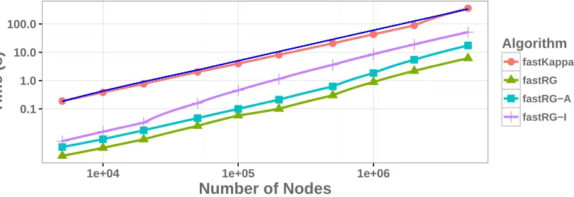
the run time experiment that was performed in Hagberg and Lemons (2015). This simulation is for an Erd˝os-R´enyi graph with expected degree 10, forn ranging between 5,000 and 5M. Speed comparisons are troubled by the fact that our code returns an edge list inRand f ast-κ returns a

● ● ● ● ● ● ● ● ● ● ● ● ● ● ● ● ● ● ● ● ● ● ● ● ● ● ● ● ● ● ● ● ● ● ● ● ● ● ● ● ● ● ● ● ● ● ● ● ● ● ● ● ● ● ● ● ● ● ● ● ● ● ● ● ● ● ● ● ● ● ● ● ● ● ● ● ● ● ● ● ● ● ● ● ● ● ● ● ● ● ● ● ● ● ● ● ● ● ● ● 0.1 10.0 1e+06 1e+08 E(m) time log10(n) 7 6.67 6.33 6 5.67 5.33 5 4.67 4.33 4 Fixing n, the running time appears to grow linearly with E(m)

● ● ● ● ● ● ● ● ● ● ● ● ● ● ● ● ● ● ● ● ● ● ● ● ● ● ● ● ● ● ● ● ● ● ● ● ● ● ● ● ● ● ● ● ● ● ● ● ● ● ● ● ● ● ● ● ● ● ● ● ● ● ● ● ● ● ● ● ● ● ● ● ● ● ● ● ● ● ● ● ● ● ● ● ● ● ● ● ● ● ● ● ● ● ● ● ● ● ● ● 0.1 10.0 1e+05 1e+07 n time log10(E(m)) 8 7.67 7.33 7 6.67 6.33 6 5.67 5.33 5 Fixing E(m), the running time appears to grow linearly with n

Figure 1: Both plots present the same experimental data. In the left plot, each line corresponds to a different value ofnand they are presented as a function ofE(m). In the right plot, each line corresponds to a different value ofE(m)and they are presented as a function ofn. On the right side of both plots, the lines start to align with the solid black line, suggesting a linear dependence onE(m)andn.

withfastRG. There are three lines in Figure 2 forfastRG, one line for each data type (edge list, sparse adjacency matrix, and igraph). The speed comparison in Figure 2 corresponds to the average running time over 10 simulations performed on a 2015 MacBook Pro, 2.8 GHz Intel Core i7, with 16 GB 1600 MHz DDR3 running Python 3.5.2 andR3.3.2. The slope of the blue line corresponds to the running timeO(nlogn). While none of these packages have been optimized for speed, they are all sufficiently fast for a wide range of purposes.

3.3. Simulating small and dense graphs withfastRG

This section investigates the graph density at whichfastRGbecomes slower than simulating each elementAi j as a Bernoulli random variable. In Figure 3, the reported time to compute this naive

(element-wise) algorithm includes both (i) the time it takes to compute the probabilities eA = X%*%B%*%t(X)and (ii) sample the edgesz = rbinom(length(eA), 1, eA). The time for fastRGis for a directed graph, represented as a sparse matrix. The time to computefastRGalso includes the time it takes to constructXandB.

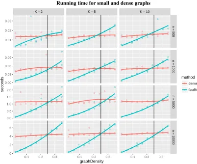
Figure 3 compares these two approaches on a set of Stochastic Blockmodels for values K∈ {2,5,10},n∈ {500,1000,5000,10000}, and graph densityρ=n−2E(m)varying between.02 and

.35. In all simulations, theS matrix is proportional to IK+JK∈RK×K, where IK is the identity

matrix andJK is the matrix of ones. The scale ofSis adjusted to ensure the correct densityρ. For

Running time offastRGand f ast-κon Erd˝os-R´enyi graph with expected degree 10

● ●

●

● ●

●

● ●

●

●

0.1 1.0 10.0 100.0

1e+04 1e+05 1e+06

Number of Nodes

Time (s)

Algorithm

● fastKappa

fastRG

fastRG−A

fastRG−I

Figure 2: As the number of nodes increases (horizontal axis), all of the running times increase in parallel to the solid blue line which gives the rateO(nlogn). The bottom three lines all correspond tofastRG, outputting three different graph types (edge list, sparse adjacency matrix, and igraph). For example, in roughly 8 seconds, f ast-κ generates a graph with 20k nodes andfastRGgenerates an igraph with 1M nodes. To generate the random edge list on 1M nodes withfastRGtakes less than 1 second

approximately the crossover point in all simulations. For scale, ρ=.25 corresponds to expected

degrees 125, 250, 1250, and 2,500 respectively fornvalues 500,1000,5000,and 10000.

Acknowledgments

This research was supported by NSF grant DMS-1612456 and ARO grant W911NF-15-1-0423.

Appendix A. Proofs

For an integerd, define 1d∈Rdas a vector of ones. The proof of Theorem 4 requires the following

lemma, which says that a vector (or matrix) of independent Poisson entries becomes multinomial when you condition on the sum of the vector (or matrix).

Lemma 8 Let A∈_Rn×n_{be the random matrix whose i,jth element A} i j

i.d.

∼ Pois(λi j)i,j=1, . . . , n.

Then conditioned on∑i,jAi j=1TnA1n=m,

(A11,A12, . . . , Ann)∼Multinomial(m, λ/

_∑

i j

Running time for small and dense graphs

K = 2 K = 5 K = 10

0.01 0.02 0.03

0.00 0.03 0.06 0.09

0.0 0.5 1.0 1.5 2.0

0 2 4 6

n = 500

n = 1000

n = 5000

n = 10000

0.1 0.2 0.3 0.1 0.2 0.3 0.1 0.2 0.3

graphDensity

seconds

method

denseRG

fastRG

Figure 3: This figure compares the run time offastRGto the run time of simulating eachAi j as a

Bernoulli random variable (denseRGin the legend). Note that the number of edges grows quadratically with the edge density. So, as the density of the graph increases (horizontal axis), the running time offastRGgrows quadratically, whereas the running time of the naive algorithm does not depend on the density of the graph. In this simulation, the crossover is aroundρ=.25 (black line). This figure shows that even for relatively small

whereλ= (λ11,λ12, . . . , λnn). That is, let a∈Rn×nbe a fixed matrix of integers with1Tna1n=m,

then

P(A=a|1TnA1n=m) = P(A11=a11,A12=a12, . . . , Ann=ann|1TnA1n=m)

= m!

∏i,jai j!

∏

λi j

λ11+λ12+· · ·+λnn

ai j

.

For completeness, a proof of this classical result is given at the end of the paper. The next proof is a proof of Theorem 4.

Proof LetAcome from the Poisson gRPG withX andSand identity mean function. Let ˜Abe a sample fromfastRG. For any fixed adjacency matrixa, we will show thatP(A=a) =P(A˜ =a).

Definem=1Tna1nand decompose the probabilities,

P(A=a) = P(1TnA1n=m)P(A=a|1TnA1n=m) (1)

P(A˜=a) = P(1TnA˜1n=m)P(A˜=a|1nTA˜1n=m). (2)

The proof will be divided into two parts. The first part shows thatP(1TnA1n=m) =P(1TnA˜1n=m)

and the second part will show thatP(A=a|1TnA1n=m) =P(A˜=a|1TnA˜1n=m).

Part 1: The sum of independent Poisson variables is still Poisson,

∑

i j

Ai j∼Poisson(

∑

λi j).

So, we must only show that 1TnA1nand 1TnA˜1nhave the same Poisson parameter:

∑

i j

λi j=1TnX SX1n=1TnXCC

−1

SC−1CX1n=1TnX˜S˜X˜1n=1TnX˜S˜X˜1n=1TKS˜1K=

∑

˜

Suv.

Part 2: After conditioning on 1TnA1n=m, Lemma 8 shows thatAhas the multinomial

distribu-tion. InfastRG, we first sample 1TnA˜1nand then add edges with the multinomial distribution. So,

we must only show that the multinomial edge probabilities are equal forAand ˜A. From Lemma 8, the multinomial edge probabilities for A are λi j/∑a,bλab. To compute the multinomial edge

probabilities for ˜A, recall that(I,J)is a single edge added to the graph infastRG. By Theorem 1,

P(A˜i j=1|1TnA˜1n=1) =P (I,J) = (i,j)=

hxi,xjiS

∑a,bhxa,xbiS

= λi j

∑a,bλab

This concludes the proof.

Proof[Proof of Theorem 7] LetUi j i.i.d

∼ U ni f orm(0,1). DefineA andB:

Ai j=1(Ui j>1−e−λi j),

Note thatA andBare equal in distribution tot(A˜)andBrespectively. By Taylor expansion,

EkA −Bk2_F =

_∑

i,j

(λi j−(1−e−λi j)) =

_∑

∞

∑

k=2

(−λi j)k/k!=

_∑

O(λi j2) =

∑

O((αn/n)2) =O(αn2).

Then,EkBk2

F =∑i jλi j>cαnn. So, definingt(A˜)andBwith the above coupling yields the result.

Proof[proof of Lemma 1]

P(A=a|1TnA1n=m) = P

(A=a)

P(1TnA1n=m)

=

∏i,j

λ_{i j}ai j

ai j!

e−λi j

(λ11+λ12+· · ·+λnn)m

m! e

−(λ11+λ12+···+λnn)

= m!

∏i,jai j!

∏

λi j

λ11+λ12+· · ·+λnn

ai j

References

E Airoldi, E Blei, S Fienberg, and E Xing. Mixed membership stochastic blockmodels. Journal of Machine Learning Research, 9(5):1981–2014, 2008.

D Cai, T Campbell, and T Broderick. Edge-exchangeable graphs and sparsity. In Advances in Neural Information Processing Systems, pages 4242–4250, 2016.

H Crane and W Dempsey. Edge exchangeable models for network data. arXiv preprint arXiv:1603.04571, 2016.

A Hagberg and N Lemons. Fast generation of sparse random kernel graphs. PloS one, 10(9): e0135177, 2015.

T Herlau, M Schmidt, and M Mø rup. Completely random measures for modelling block-structured sparse networks. InAdvances in Neural Information Processing Systems 29. 2016.

P Holland, K Laskey, and S Leinhardt. Stochastic blockmodels: First steps. Social Networks, 5(2): 109–137, 1983.

B Karrer and M Newman. Stochastic blockmodels and community structure in networks. Phys. Rev. E, 83:016107, Jan 2011.

P Latouche and C Ambroise. Overlapping stochastic block models with application to the french political blogosphere. Annals of Applied Statistics, 5(1):309–336, 2011.

A Todeschini and F Caron. Exchangeable Random Measures for Sparse and Modular Graphs with Overlapping Communities. arXiv preprint arXiv:1602.02114, February 2016.

M Vose. A linear algorithm for generating random numbers with a given distribution. IEEE Trans-actions on software engineering, 17(9):972–975, 1991.

A Walker. An efficient method for generating discrete random variables with general distributions.

ACM Transactions on Mathematical Software, 3(3):253–256, 1977.