Two-dimensional linear prediction model-based decorrelation method

(1)

MURDOCH RESEARCH REPOSITORY

http://dx.doi.org/10.1109/34.24801

Lin, Z. and Attikiouzel, Y. (1989) Two-dimensional linear

prediction model-based decorrelation method. IEEE

Transactions on Pattern Analysis and Machine Intelligence,

11 (6). pp. 661-665.

http://researchrepository.murdoch.edu.au/19349/

Copyright © 1989 IEEE

Personal use of this material is permitted. However, permission to reprint/republish

this material for advertising or promotional purposes or for creating new collective

(2)

tions a =

i,

dl 2 do is equivalent to

k l f ( f + 1 ) 2 2 ( f - I )

+

C , ( f + 1) w h e r e 6 = ( f - l ) a ,

1

+

6

+

( g

+

1 ) - . ( A . 1 0 ) 2

6)-1

Let 4 = f - I , y = g - 1. Then after tedious algebra, it can be shown that ( A . IO) is equivalent to the inequality

[ - d 2 - 104

-

4y

+

2 y ]

42u2

+

[34*

+

~ I # I ~ -‘64 + 74

+

271 U

+

2 d 2 2 0. ( A . l l ) Recombining the terms of the left-hand side of ( A . 1 I ) , it becomes

( y - 4 u - T U ) d13a

+

42a[34

+

y - 104a

+

2 y a ]

+

2(r#I2 - 2 4 2 a

+

y 4 a ) .

Since

11

ho

I/

=

1)

go

)I

implies + U = y b , the three terms of the above can be expressed as

y - C#XX - ~ C X = y ( 1 - U ) - $ U 2 y b - 4 b = 0, 34

+

y - 1 0 4 ~

+

2 y a 2 2 4 ( 1 - b - U )

+

4 ( l

- 2 a )

+

y ( l - 2 b ) 2 0,

4 2

- 3d2a

+

r4a

2 4 ( l - b - U ) 2 0.

The theorem is proven. The equality holds when 1) 4 = y = 0, i.e., both Xo and Yo are white noise, or 2) a = b =

4.

ACKNOWLEDGMENT

The authors would like to express their sincere thanks to Dr. A . F. Petty, Dr. I . Jurkevich, and Dr. J . S. Lee for their help in data collection and computing, and for their stimulating discussions.

REFERENCES

L. Van Gool, P. Dewaele, and A. Oosterlinck, “Texture analysis anno 1983,” Comput. Vision, Graphics Image Processing, vol. 29, pp. 336-357, 1985.

A . Rosenfeld, “Survey, picture processing, 1985,” Compur. Vision, Graphics, Signal Processing, vol. 34, pp. 204-251, 1985. J . T. Tou, “Pictural feature extraction and recognition via image modeling,” in Image Modeling, A. Rosenfeld, Ed. 1981, pp. 391- 421.

A. K. Jain, “Partial differential equations and finite-difference models

in imaging processing, Part 1: Image representation,” J . Optimiz. Theory Appl., vol. 23, pp. 65-91, 1977.

- , “Advances in mathematical models for image processing.”

Proc. IEEE, vol. 69, pp. 502-528, 1981.

E. J. Delp, R. L. Kashyap, and 0. R. Mitchell, “Image data compression using autoregression times series model,’’ Patrern Rec- ognitionLetr., vol. 11, pp. 313-323, 1979.

R. L. Kashyap, “Characterization and estimation of two-dimensional ARMA models,’’ IEEE Trans. Inform. Theory, vol. IT-30, pp. 736- 745, 1984.

R. L. Kashyap and A. Khotanzad, “A model-based method for ro-

tation invariant texture classification,” IEEE Trans. Pattern Anal. Machine Intell., vol. PAMI-8, pp. 472-481, 1986.

R. M. Haralick, “Statistical and structural approach to texture,” Proc. IEEE, vol. 67, pp. 786-804, 1979.

C. W. Therrien, “An estimation-theoretic approach to terrain image segmentation,” Comput. Vision, Graphics, Image Processing, vol.

C. W. Therrien, T . F. Quatieri, and D. E. Dudgeon, “Statistical model-based algorithms for image analysis,” Proc. IEEE, vol. 74,

G. R. Cross and A. K. Jain, “Markov random field texture models,”

IEEE Trans. Pattern Anal. Machine Intell., vol. PAMI-5, pp. 25-39, 1983.

22, pp. 313-326, 1983.

pp. 532-551, 1986.

R. Chellappa, and R. L. Kashyap, “Texture synthesis using 2-D noncausal autoregressive models,” IEEE Trans. Acoust., Speech, Signal Processing, vol. ASSP-33, pp. 174-203, 1985.

D. Tj$stheim, “Statistical spatial series modelling,’’ Adv. Appl. Prob., vol. 10, pp. 130-154, 1978.

R. L. Kashyap, R. Chellappa, and A. Khotanzad, “Texture classification using features derived from random field models,” Parrern Recognirion Lett., vol. 1, pp. 43-50, 1982.

B. Julesz, “Cluster formation at various perceptual levels,” Metho- dol. Pattern Recognirion, pp. 297-315, 1968.

B. Ashjari, “Computer detection and identification of a visually in- discernible texture mixture,” in Proc. IEEE Compur. Soc. Con$ Comput. Vision and Pattern Recognition, 1985, pp. 172-174. P. Diaconis and D. Freedman, “On the statistics of vision: The Julesz conjecture,” J . Math. Psycho/., vol. 24, pp. 112-138. 1981. G . E. Keyte and J. T . Macklin, “SIR-B observations of ocean waves in the NE Atlantic,” IEEE Trans. Geosci. Remote Sensing, vol. GE- 24, pp. 552-558, 1986.

T. D. Allan, Ed., Satellite Microwave Remote Sensing. New York: Wiley, 1983.

M. N. Youssef, “On the accuracy of forecasting telephone usage de- mand,” Bell Lab. Tech. J . , vol. 63, pp. 819-849, 1984.

T. Ozaki, “On the order of determination of ARIMA models,” Appl. Statisr., vol. 26, pp. 290-301, 1977.

G. E. P. Box and G. M. Jenkins, Time Series Analysis: Forecasting and Control, rev. ed.

F. M. Monaldo and D. R. Lyzenga, “On the estimation of wave slope- and height-variance spectra from SAR imagery,” IEEE Trans. Geosci. Remote Sensing, vol. GE-24, pp. 543-551, 1986.

B. Kinsman, Wind Wave. Englewood Cliffs, NJ: Prentice-Hall, 1965.

J . S . Lim and A. V. Oppenheim, “Enhancement and bandwidth compression of noisy speech,” Proc. IEEE, vol. 67, pp. 1586-1640, 1979.

H. Chang and J . K. Aggarwal, “Design of two-dimensional semi- causal recursive filters,” IEEE Trans. Circuits Syst., vol. CAS-25,

L. R. Rabiner and B. Gold, Theory and Application of Digital Pro- cessing.

J. S . Lee, “Speckle suppression and analysis for synthetic aperture radar images,” Opt. Eng., vol. 25, pp. 636-643, May 1986. W. A. Fuller, Introduction to Statisrical Time Series. New York: Wiley, 1976.

G. E. P. Box and D. A. Pierce, “Distribution of residual autocorrelations in autoregressive integrated moving average time series models,” J . Amer. Starist. Ass., vol. 65, pp. 1509-1526, 1970. A. I. Mcleod, “On the distribution of residual autocorrelations in Box-Jenkins models,’’ J . Roy. Sratist. Soc. B , vol. 40. pp. 296-302, 1978.

San Francisco: Holden-Day, 1976.

pp. 1051-1059, 1978.

Englewood Cliffs, NJ: Prentice-Hall, 1975.

Two-Dimensional Linear Prediction Model-Based

Decorrelation Method

ZHENYONG LIN A N D Y. ATTIKIOUZEL

Abstract-This correspondence presents a unified feature extraction scheme, viz. two-dimensional (2-D) linear prediction model-based de- correlation method. By applying 2-D causal linear prediction model to decorrelate a textured image, the very heavy computation load re-

quired when using whitening operator to decorrelate the image, or the

Manuscript received July 21, 1987; revised November 2, 1988. Rec- ommended for acceptance by 0. D. Faugeras. This work was supported by a research grant from the University of Western Australia.

The authors are with the Department of Electrical and Electronic En- gineering. University of Western Australia, Nedlands WA 6009, Western Australia.

IEEE Log Number 8927501.

(3)

~

662 IEEE TRANSACTIONS ON PATTERN ANALYSIS AND MACHINE INTELLIGENCE. VOL. 1 1 . NO. 6. JUNE 1989

significant information loss when using gradient operator to approxi-

matelj whiten the image ir avoided. This texture model-based decor-

relation method provides three sets of features to perform texture clas- sification: the coefficients of the 2-D linear prediction, the moments of error residuals and the autocorrelation values. An optimum feature selection scheme using modified branch-and-bound method was intro-

duced t o reduce information redundancy. After feature selection, 100

percent classification accuracy was achieved for a 20 class texture

problem. Experiments show that this feature extraction scheme is truly information lossless, effective, and fast.

Index Terms-Feature extraction, image processing, texture analy- sis.

I. INTRODUCTION

Texture is an important characteristic used in analyzing objects o r regions of interest in an image. Texture features play an important role in image classification and analysis. In classification, texture features can be used t o discriminate and label areas of an image, such as crop identification in an aerial photograph, and medical diagnosis of an X-ray photograph. Texture features can also b e used in scene segmentation and identification in a n image under- standing or computer vision system, for example, in robot vision and industrial inspection. Therefore, the choice of texture features is the key in these applications.

Currently, there are a lot of approaches to choosing texture features. Some of these based on statistical techniques are: Fourier power spectrum [2], gray level run length [2], [6], Gray level difference [2], gray level co-occurrence matrices [ l ] , [2], 171, [8], decorrelation method 131, and visually perceived properties [9]. Some of these based on parametric models are mosaic model [ l o ] , autoregressive model (AR) [ I 11, [13], [22], and Markov random field (MRF) model 1121. [14].

The motivation of this correspondence is to unify the parametric model-based approach with the statistical technique based approach for choosing texture features, viz. the 2-D linear prediction model-based decorrelation method. In the original decorrelation method of feature extraction [3]. there are two major disadvan- tages: the computation of the autocorrelation shape features, o r the use of a whitening operator to decorrelate the textured image, is computationally very expensive; some information will be lost in the whitening process, especially if one uses a gradient operator, such as the Laplacian o r Sobel operator, to approximate the whitening operator. According to [ 141, the information loss is significant because the error residuals themselves contain only partial infomiation of the original image. Due to these t w o reasons, it is not viable to use a decorrelation method in any practical situation. A 2-D linear prediction model [15]-[17], [20] was widely used i n many aspects of image analysis, for example, in image coding [ 17) and segmentation [ I S ] . T h e two-dimensional autoregressive model, which is closely related t o 2-D linear prediction model, was also used in texture classification [ l I ] , [13], [22]. O u r objective in this paper is to use a 2-D causal linear prediction model to whiten a textured image to overcome the two drawbacks in the decorrelation method, thus making this feature extraction scheme much faster and information lossless. This can be achieved because the coefficients of the 2-D linear prediction model provide us with ex- tra and very important information about texture, and its computation is fast. Note that the noncausal simultaneous autoregressive model (SAR) in [221 can also be used to whiten a textured image when using maximum likelihood estimation technique. However, the estimation of the 2-D linear prediction model involves only an inversion of a block Toeplitz autocorrelation matrix, and its computation is simpler and faster than the interative estimation scheme of the SAR model.

A Gaussian M R F model was also used for texture classification [I41 and excellent results were obtained. Although the 2-D linear prediction model is a special case of the M R F model and SAR

models under Gaussian assumption, for non-Gaussian textures, the probability structure of these models is different, and further problems may be posed to these t w o models for non-Gaussian textures o r highly structured o r macrotextures. Both [14] and [22] did not fully utilize information from the error field while the feature extracted from white noise field is a key feature as we will see from our experiment.

O u r second modification to the original decorrelation method is

to use autocorrelation values directly a s features, as suggested in [ 141. Because autocorrelation values themselves carry out enough texture information, it is not necessary to perform the time con- suming autocorrelation shape feature calculation. This further sim- plifies the original method. With these two major modifications, our feature extraction scheme has proven a much faster and more powerful method. It produces a true information lossless feature set.

11. 2-D LINEAR PREDICTION MODELS

Two-dimensional linear prediction models have been widely re- ported in the literature [15], 1171. Consider x ( m , r z ) as a sample of a 2-D sequence of intensity image with rn and n range over some finite lattices. The random field variable can then be represented by a 2-D prediction model 1151, 1171 as:

( 1 ) x,,(rn, n ) =

cc

a ( k , j )

*

x ( r n - k , n - j )

+

i l

( h . ] )En

where lI represents the nonzero support region or mask for prediction coefficients a ( k , j ); a. represents a locally constant bias coefficient added to the input.

The prediction error is

e ( m , n ) = x ( m , n ) - .r,,(m, n )

= x ( m , n ) -

cc

a ( k , j ) * x ( m - k . n - j ) - u o . h i

( i ( . / ) E n

( 2 ) Suppose x ( m . n ) is an arbitrary stationary 2-D random field, then to minimize the variance of the prediction error,

E [ ( x ( m , n ) - x , , ( m , n ) l 2 ] ( 3 )

must be a minimum.

By varying the linear prediction coefficients a ( k , j ), minimi- zation of (3) gives a set of linear equations called the Normal equations:

C ( p , 4 ) -

xc

a ( k , j )

*

C ( p - k , 4 - j )

L J

l h . i l E n

- a.

*

XZ

x ( r n - p , n - 4 ) =

0 '

*

6 ( p , 4 ) ( 4 )

ni n

1 m. ,I 1 E w

where

0

represents the minimum variance of the error field of the 2-D linear prediction; 6 ( p , 4 ) is the two-dimensional Kronecker delta function, W is an M X

M

estimation window; C ( p , 4 ) represents the covariance Coefficients of random field { .r( m , n ) } which are estimated as:

C ( k , j ) =

cc

[I(,, r z )

*

( x ( m - k , n - J ) ) ] . _{( 5 )} nt n

I ? ? I , , ! )E w

Solving the Normal equations, the optimum coefficients of the 2-D linear prediction model can be obtained. A stochastic representation for a pixel x ( m , n ) is

x ( m , n ) = x,(rn, n )

+

e ( m . n ) . ( 6 )

For a causal mask, which is either a non symmetric half plane or

(4)

as the Cholesky decomposition [20] or the more efficient method described in [ 191. Usually in image processing applications, only a low order prediction model is required, this means that both the computation time of the covariance coefficients is less, and the cal-

TABLE 1

CLASSIFICATION RESULTS USING T H E SUB DIMENSIONAL FFATURE VECTOR

FOR (64 x 64) SIZED SUBIMAGE

culations of the prediction coefficients and moments of error resid- l 2 3 4 5 6 7 8 9 10 11 12 13 14 15 16 17 18 19 20

uals are faster.

There are three methods for calculating the coefficients of the model according to the treatment of bias, and two techniques for estimating the covariance coefficients [ 171. In this paper, the autocorrelation method was used to determine the range of summa- tion in ( 5 ) . It is assumed that the data are zero outside the ( M x M ) estimation window. The local mean linear prediction approach [17] was employed to calculate the coefficients of the 2-D linear prediction. The local mean of the data over the ( M X M ) estimation window is estimated, and is subtracted from every pixel within the ( M X M ) frame. The coefficients of the 2-D linear prediction model are then obtained by solving the normal equations (4) with- out bias.

111. CLASSIFICATION SCHEME

~ ~~

1 1 6 0 0 0 0 0 0 0 0 0 0 0 0 0 0 0 0 0 0 0

2 0 1 6 0 0 0 0 0 0 0 0 0 0 0 0 0 0 0 0 0 0

3 0 0 1 6 0 0 0 0 0 0 0 0 0 0 0 0 0 0 0 0 0

4 0 0 0 1 6 0 0 0 0 0 0 0 0 0 0 0 0 0 0 0 0

5 0 0 0 0 1 5 0 0 0 0 0 0 0 0 0 0 0 1 0 0 0

6 0 0 0 0 0 1 4 0 0 0 0 0 0 0 0 2 0 0 0 0 0

7 0 0 0 0 0 0 1 6 0 0 0 0 0 0 0 0 0 0 0 0 0

8 0 0 0 0 1 0 0 1 4 0 0 0 0 0 0 1 0 0 0 0 0

9 0 1 0 0 0 0 0 0 1 5 0 0 0 0 0 0 0 0 0 0 0

1 0 0 0 0 0 0 0 0 0 0 1 6 0 0 0 0 0 0 0 0 0 0

1 1 0 0 0 0 0 0 0 0 0 0 1 6 0 0 0 0 0 0 0 0 0

1 2 0 0 0 0 0 0 0 0 0 0 0 1 5 0 0 0 0 0 0 1 0

1 3 0 0 0 0 0 0 0 0 0 0 0 0 1 6 0 0 0 0 0 0 0

1 4 0 0 0 0 0 0 0 0 0 0 0 0 0 1 6 0 0 0 0 0 0

In this application, a 3 X 3 quarter-plane prediction mask, i.e., 15 0 0 0 0 0 0 0 0 0 0 0 0 0 0 16 0 0 0 0 0

an 8th o r d e r 2 - D linearprediction model, was chosen. The 8 coef- 16 0 0 0 0 0 0 0 0 0 0 0 0 0 0 0 1 6 0 0 0 0

ficients of the 2-D linear prediction and the moments of error re- 17 0 O O O 1 0 0 0 0 0 0 0 0 0 0 0 15 0 0 0

siduals were chosen as features. The features that were derived 18 0 0 0 O 0 0 0 0 0 0 0 0 0 0 0 0 0 16 0 0

from the error residuals are: variance /3, skewness, and Kurtosis 19 0 0 0 O 0 0 0 0 0 0 0 0 0 0 0 O 0 0 16 0

[3], [18]. As the coefficient s o f t h e 3 X 3 quarter-plane2-Dlinear 2o O O O O O O l 6 prediction were extracted from autocorrelation values C ( K , j ),

formation contained in these There is no point in choosing these autocorrelation values as features. Therefore the additional autocorrelation values C ( K . i ( K = -3. 3. i = 0. 1. 2: K = -3.

with K = -2, -1,

. . .

2 , and j = 0, 1, 2, they cover most in- M;sclass$cation: 8 out of 320.

Note: NudXx's 1-20 represent D68, D9, D84, D24, D19. D92. D12,

D112, D29, D17, D4, D57, D77, D36, D38, D15, D2, D65, D3, D95 in Brodatz, respective,y,

~ " , ~

- 2 ,

. . .

3 , j = 3 ) required for 4 X 4 quarter-plane 2-D linear prediction were chosen as features. Since C ( -3, 0 ) = C ( 3 , O ) , there were only 12 autocorrelation values. These values were nor- malized by dividing by C ( 0 , 0 ) as suggested in [14]. The above three sets of features give a feature vector with 23 components.

Having chosen features, we can adopt a Bayes decision rule o r other standard rules for classification. A minimum distance classifier [14], [22] was chosen because of its simplicity and less computation requirements, which is especially important in the later feature selection stage. It can be described as

n

d ( X ' " , i ) =

c

[ X ' " ( f ) - p y f ) ] 2 / ( 7 ( f ) ( f ) . _{( 7 )}

f = l

First, the feature mean P I ' ) ( f ) and variance U ( ' ) ( f ) were calcu-

lated for each feature c o m p o n e n t f (

f

= 1, 2,

. . .

n , n is feature dimension) of every class i ( i = 1, 2 ,

. . .

K , K is class number). A "leave-one-out" strategy was adopted, i.e., to take out a spe- cific feature vector from a class as test sample X " ) , the remaining feature vectors in that class and all the feature vectors in other classes were used to train the classifier, i . e . , the mean p ( f ) and variance a( f ) were recomputed for that class using the remaining feature vectors from it. After calculating distance from X ( ' ) to every class, the test sample Xi') was then assigned to a class i* for which the distance in (7) is a minimum. This was repeated for every sample of each class.

IV. EXPERIMENT RESULTS

We often find that many feature extraction schemes perform classification well, but with only a small group of textures. When texture classes are increased, especially when macrotextures are included, the classification accuracy drops quite a lot. Therefore, in our experiment, we chose 2 0 classes of textures from Brodatz [4], including both microtextures and macrotextures, to test ro- bustness of our scheme. The number of these textures are: D68, D9, D84, D24, D19, D92, D12, D112, D29, D17, D 4 , D57, D77, D36, D38, D15, D2, D65, D3, D95. Each texture was digitized into a ( 5 12 X 5 12 ) image by a PC vision board installed in an IBM

AT computer. These images were further reduced to a ( 2 5 6 X 2 5 6 ) resolution by averaging every four pixels. Each image was then subdivided into 16 subimages of ( 6 4 X 6 4 ) size with one column overlap. Thus each texture class had 16 samples.

In order to make feature vector invariant to illumination changes, hence increasing classification accuracy, some commonly used preprocessing techniques were adopted. First, a histogram equali- zation over each subimage was performed. Then normalizing cach subimage into a zero empirical mean and unit empirical variance was carried out. After preprocessing, the feature vectors mentioned in Section 111 were calculated. Classification experiment was con- ducted using these 23 features and minimum distance classifier. The results are shown in Table I. Classification accuracy is 9 7 . 5 percent.

V . F E A T U R E S E L E C T I O N

From experimental results we can see that our feature extraction scheme is powerful. But there still exist some problems: the information contained in the feature set is redundant, and some features in the set make classification accuracy worse, instead of making a contribution to it; the feature dimension is still too high. High dimension requires longer computation time and more memory space, it also makes the design of the classifier difficult if one wants to use an advanced classifier, such as the Bayes classifier in [22]. Furthermore it makes classification process slow, and not suitable for real time identification. Also, in some cases one might want classification accuracy as high as possible, for example, in medical diagnosis. For all above reasons, it is necessary to design an optimal feature selection scheme to reduce the feature dimension. Al- though the computation might be heavy in this process, because it

is an off-line computation, once optimum feature set has been found, the calculation of this set and classification using this set will be much faster.

(5)

664 IEEE TRANSACTIONS ON PATTERN ANALYSIS A N D MACHINE INTELLIGENCE. VOL I I . NO 6. J U N E 19x9

Define a binary-valued solution vector A a s

where I I is equal to the feature dimension and t represents the vector transposition.

The minimum distance classifier can be transformed into the fol- lowing expression:

where uI = 1 means that t h e j t h feature component has been se- lected; a , = 0 means it has been excluded.

Define an assignment matrix A F . for test data x ' ' ) of class k ( k = I , 2 ,

. .

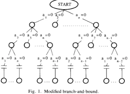
. 2 0 ) . If the i t h distance d ( u " ' , i ) is minimum, then the i t h column in the kth row will be increased by one, i.e., assign class k to class i. T h c diagonal elements of A F will then represent the number correctly classified. The total classification accuracy will be the trace of A F . T R ( A F ) . The feature selection problem now becomes: to find the value of vector A to maximize T R ( A F ) . Obviously, this is a zero-one unconstrained nonlinear integer pro- gramming problem. A modified branch-and-bound algorithm was designed to solve this problem efficiently. The algorithm is as follows.

Step 1: For each of the present branches, set CJ, = 0 f o r j = 1, 2 ,

. . . I I ,

and j not being included in the branch record, calculate the corrcsponding TR ( A F ) and store it in a matrix B which records both the branch which is under processing and the classification accuracy aftcr the j t h component of features is masked off in that branch, i.e., let [ I , = 0. So each present branch has many sub-

branches.

Srep 2: Find the maximum classification accuracy of all the subbranches just obtained and stored in matrix B .

Step 3: If the maximum classification accuracy of the subbranches is larger than o r equal to that of the present branch then continue to Step 4, else stop.

Step 4: The maximum classification accuracy is used as the low bound. Any subbranch which has classification accuracy lower than the maximum will be discarded. The branch record will record only the subbranches which have maximum classification accuracy. Go

The schematic diagram of this algorithm is represented by the tree in Fig. 1.

Note that branches aI, a,,, a?, a,,, a , , a? and a l . a?, a,, represent the same set of features. So at each branch level, those branches which represent the same set of features but with different feature sequence should b e reduced to one branch so as t o increase computation efficiency.

Comrnent: This algorithm is a tradeoff between branch-and- bound algorithm and sequential backward selection (SBS) algorithm [21]. It overcomes the large amount of computation still required in the branch-and-bound algorithm, thus making it computationally feasible. and it also partially eliminates the drawbacks in the SBS algorithm. i . e . , once some feature components have been discarded, it does not allow any revision of their merit. In the pre- sented algorithm, if a feature component is discarded in one branch,

it can be assessed by other branches. Therefore the algorithm will get optimum or near-optimum feature sets.

Above feature selection scheme was applied to the 23 dimensional feature vectors calculated in Section IV. Nine optimum feature sets were obtained with feature dimension of 13, 12, I I , I O , 9. respectively, each with 100 percent classification accuracy.

During the feature selection process. the classification accuracy was nondecrease until reaching 100 percent. When proceeded further after reaching 100 percent accuracy with dimension of 9, the accuracy decreased monotonically. Hence, we got a group of key features (from most important to least important): a [ O , I ] , Kur- tosis. C [ 2 , 31, C [ -3, 21. a [ O , 2 ) . a I 2 , 01. Taking out any one of these will make significant decrease of classification accuracy. to Stcp 1.

a = O

92

a.=O

=o

= O

n - I

Fig. 1 . Modified branch-and-bound

In order to choose the best feature set from the nine groups, the same 2 0 classes of textures in Brodatz album were resampled with lower illumination condition and different area. The samples in the first group were used to train the minimum distance classifier with different feature set in the nine optimum groups. The samples in the second group were used as test samples. T w o groups of the optimum feature set with dimension 13 misclassified only 2 samples of Field stone ( D 2 ) into Bubbles ( D 1 1 2 ) . The remaining groups misclassified 3 samples of D2 into DI 12, all yielding classification accuracy of over 99 percent. This error is mainly due t o the Field stone picture in Brodatz containing more dark holes, especially the area near the edge of the photograph, and lower illu- minance condition. The best feature set, according to classification accuracy, is composed o f a [ I , 01, a [ 2 , 0 ] , a [ O , I ] , a [ I , I ] , a [ 2 , I ] , a [ O , 21,

0,

Skewness, Kurtosis, C ( -3, 2 ) , C ( -3, 3 ) , C ( 2 , 3 ) . C ( 3 , 0 ) o r C ( 3 , 1 ) .

VI. S U M M A R Y A N D CONCLUSION

Experimental results show that this unified method is a true information lossless feature extraction scheme. It is more powerful than any single parametric model based approach o r statistical technique based approach.

Because the computation of the coefficients of the 2-D linear prediction is fast, it is the cheapest white noise driven model, and therefore, makes this modified decorrelation method efficient, loss- less and practical.

This scheme is suitable to a variety of textures, from microtex- ture to macrotextures. Therefore, it has a wide range of applications.

Experiments carried on an Intel 80386 C P U based computer Apricot VX show that the feature selection scheme given in this correspondence is suitable t o feature dimension less than 30 with 2 0 classes. For higher feature dimension, one needs either to divide the feature vector into several groups o r use a higher performance computer.

ACKNOWLEDGMENT

The authors wish to thank S . Chan and E. Lai for their help and F. Fung and K. K . Ly for their valuable suggestions and discus- sion.

REFERENCES

[ I ] R . M . Haralick. "Statistical and structural approach to textures,"

Proc. IEEE, vol. 67, pp. 786-804. May 1979.

121 J . Weszka, C. R . Dyer, and A . Rosenfeld, "A comparative study of

texture measures for terrain classification," IEEE Trans. Sysr., Man. Cybern., vol. SMC-6. pp. 269-289, Apr. 1976.

[31 0. D. Faugeras and W . K. Pratt, "Decorrelation methods of texture feature extraction." IEEE Trans. Pattern Anal. Machine Inre//. , vol.

[41 P. Brodatz, Texture: A Photographic Album f o r Artists and Design-

PAMl-2. pp. 323-332, July 1980.

(6)

C. H . Chen, “A study of texture classification using spectral features,” in Proc. IEEE 6th Ini. Con$ Pattern Recogniiion, Munich, Germany, Oct. 19-22, 1982, pp. 1074-1077.

M. Galloway, “Texture analysis using gray-level-run lengths,” Compui. Graphics, Image Processing, vol. 4, pp. 172-199, 1974. R. M. Haralick, K. Shanmugam, and I. Dinstein, “Textural features for image classification,” IEEE Trans. Syst., Man, C.vbern., vol.

L . S . Davis, S . Johns, and J . K. Aggrawal. “Texture analysis using generalized co-occurrence matrices, ” IEEE Trans. Pattern Anal. Ma-

chine Intell,, vol. PAMI-l, pp. 251-259, July 1979.

H . Tamara, S . Mori, and T. Yamawaki, “Texture features corre-

sponding to visual perception,” IEEE Trcms. Sysi.. Marl, Cybern.. vol. SMC-8, pp. 460-473, June 1978.

N. Ahuja and A. Rosenfeld, “Mosaic models for texturers,” IEEE Trans. Paitern. Anal. Machine Iniell., vol. PAMI-3, pp. 1 - 1 I , 1981. P. De Souza, “Texture recognition via autoregression.” Pattern Rec-

ogniiion, vol. 15, pp. 471-475, 1982.

0. R. Cross and A. K. Jain, “Markov random field texture models,” IEEE Trans. Paiiern. Anal. Mtichine Iniell.. vol. PAMI-5, pp. 25- 39, 1983.

R. L. Kashyap and A. Khotanzad, “A model-based method for ro-

tation invariant texture classification,” IEEE Trans. Pattern Anal. Machine Iniell,, vol. PAMI-8, pp. 472-481. July 1986.

R. Chellappa and S . Chatterjee. “Classification of textures using Gaussian Markov random fields,” IEEE Tram. Acoust., Speech, Sig- nal Processing, vol. ASSP-33, pp. 959-963, 1985.

C. W. Therrien, F. Outieri, and D. E. Dudgeon, “Statistical model- based algorithm for image analysis,” Proc. IEEE, vol. 74, pp. 532- 551. 1986.

S. Ranganatn and A. K. Jain, “Two-dimensional linear prediction models-Part I: Spectral factorization and realization,” IEEE Trans. Acoust., Speech, Signal Processing. vol. ASSP-33, pp. 280-299,

1985.

P. A. Maragos, R. W. Schafer, and R. M. Mersereau, “Two-dimensional linear prediction and its application to adaptlve predictive coding of images,“ IEEE Trans. Acousi., Speech, Slgnal Processing, vol. ASSP-32, pp. 1213-1229, 1984.

W. K. Pratt, Digiral Image Processing.

M. Wax and T . Kailath, “Efficient inversion of Toeplitz-block Toe- plitz matrix,” IEEE Trans. Acoust., Speech, Signal Processing, vol. ASSP-31. no. 5 , 1983.

L . R. Rabiner and R. W. Schafer, Digiicrl Processing ojSpeech Sig- nals.

Handbook of Pattern Recognition and Image Processing. New York: Academic, 1986.

R. L. Kashyap, R. Chellappa, and A . Khotanzad, “Texture classiti- cation using features derived from random field models,” Paiiern Recogniiion Lett., vol. I , Oct. 1982.

SMC-3, pp. 610-621, NOV. 1973.

New York: Wiley, 1978.

Englewood Cliffs, NJ: Prentice-Hall, 1978.

Efficient Parallel Algorithms for Image Template

Matching on Hypercube SIMD Machines

V. K. PRASANNA KUMAR A N D VENKATESH KRISHNAN

Abstract-In this correspondence, we present efficient parallel al- gorithms for image template matching on hypercube SIMD machines

of sizes N’, N’ x M’, and N 2 x K’ processing elements. For an N X

N image and M x M window with N * PE’s, we present a simple optimal

parallel algorithm with O ( M ’

+

log N ) time. The N’ X M’ PE’s case

Manuscript received October I O , 1986; revised November 3, 1988. This work was supported in part by NSF Grant IRI-8710836 and by grants from the U.S.C. Faculty Research and Innovation Fund and the Powell Foun- dation.

The authors are with the Department of Electrical Engineering-Sys- terns, University of Southern California, Los Angeles, CA 90089.

IEEE Log Number 8926699.

is solved in 0 ( l o g N ) time and the N’ x K 2 PE’s case is solved in

U ( M 2 / K 2

+

log N ) time. We also design a parallel algorithm for the

N 2 PE’s case using constant space/PE which runs in 0 ( M 2

*

log* ( M )

+

log N ) time. All these algorithms have superior time performance

compared to known results.

Index Terms-Hypercube, image processing, parallel algorithm,

template matching.

I. INTRODUCTION

Template matching is a basic operation in image processing and computer vision. It is used as a simple method for filtering, edge detection, image registration, and object detection. Template matching can be described as comparing a template (window) with all the possible windows of the image. Each position of the image will store the result of the window operation for which it is the top- left corner. Let

IMAGE(i,

j ) represent an N X N image where i, j E [0, N - I ] . Let W ( s , t ) represent the template where s, t E

[0, M - 11. Then the result C ( i , j ) , 0 5 i , j I N - 1 is as given below:

M - l M - I

C(i, j ) =

c

I M A G E ( ( i

+

s) mod N , ( j

+

t ) c = o r = o

.

mod N )

*

W ( s , t ) . _{( 1 )}

Note that the computation can be done in O ( N 2 X M 2 ) time using a uniprocessor.

In this correspondence, we develop simple efficient parallel algorithms for template matching on hypercube arrays of various sizes. The results include image template matching on a hypercube with N 2 PE’s in O ( M 2

+

log N ) time. The storage space available in each PE is assumed to be O ( M ) . We also present an algorithm for a hypercube with N’ X M 2 PE’s taking O ( l o g N ) time. This assumes constant storage space in each PE. The N 2 X K 2 PE’s algorithm is implemented in O ( M 2 / K 2

+

log N ) time. The storage in each P E is O ( M / K ) . We also show that these algorithms are optimal. Previous time bounds for the above three cases are O ( M

*

max ( M , log N ) ) , O ( l o g N

*

log M ) , and O ( M Z / K 2

+

(log N

*

log K ) ) , respectively [ l ] , [2]. We also design a parallel algorithm for the

N’

PE case using constant s p a c e / P E which runs in O ( M ’

*

log* ( M )

+

log N ) ’ time. This is an attractive algorithm if the window size is large. The main contribution of this paper is in designing simple elegant parallel algorithms for template matching. These results improve on the best known bounds in the literature [ l ] , [ 2 ] and most of the solutions are optimal.

This correspondence is organized as follows. In the next section, we define the hypercube architecture and discuss some of its useful properties. We also define some data movement operations which will be used in our parallel algorithms. Section I11 deals with parallel algorithms for various cases and their optimality . Conipari- sons to known results are made in the last section.

11. A HYPERCUBE SIMD MODEL

A hypercube SIMD computer is comprised of N = 2” processing elements (PE’s), each having some local memory. The PE’s are indexed 0 through N - 1 and the pth PE is referred to as PE ( p ) . All the PE’s are synchronized and operate under the control of a single instruction stream. The PE’s have enable/disable masks and a subset of PE’s can be made to execute an instruction. The set of

enabled PE’s can be changed from instruction to instruction. Each PE has a local memory of size I , an A L U , a memory address register, temporary registers, a mask bit register, and an index register. The index register of PE ( p ) stores the index p of the PE.

The PE’s are interconnected to provide inter-PE communica-

‘log* M = min { KI log log log .

. . K

times ( M ) 5 I }