Ann. Geophys., 26, 281–293, 2008 www.ann-geophys.net/26/281/2008/ © European Geosciences Union 2008
Annales
Geophysicae
Comparison of simulated and observed large-scale, field-aligned
current structures
P. Nenovski
Geophysical Institute, Bulgarian Academy of Sciences, 1113 Sofia, Bulgaria
Received: 22 January 2007 – Revised: 23 October 2007 – Accepted: 12 November 2007 – Published: 26 February 2008
Abstract. Recently, a model of large-scale, field-aligned cur-rent (FAC) structures, based on zero-frequency MHD sur-face wave (SW) modes that can emerge from the solar wind-Earth’s magnetosphere interaction, has been proposed. The FAC polarity and intensity distribution are quantified as a function of the solar wind parameters and the interplanetary magnetic field (IMF) magnitude that enter as input param-eters. Besides, there are input parameters intrinsic to the Earth’s magnetosphere – the size of the polar cap and the boundary regions and their plasma density variations. In-fluence of the IMFBy component on the FAC structure is
examined here. Depending on the IMFBy magnitude, the
predicted six-cell FAC structure tends to evolve in a spiral-like fashion. This large-scale FAC model is compared with experimental evidences and empirical FAC models based on DE-2 satellite data and high-precision Oersted and Magsat satellite magnetometer data. Among the various achieve-ments of these long-term satellite measureachieve-ments, an obser-vation/discovery of a ground-based state of FACs which in-cludes a pair of large-scale FACs in the polar cap under both positive and negative IMFBzhas been pointed out. The FAC
pattern is qualitatively and quantitatively consistent with ex-perimental data for both polar cap FAC and Region 1 and Region 2 FAC systems.
Keywords. Magnetospheric physics (Solar-wind-magnetosphere interactions; MHD waves and instabilities) – Ionosphrer (Electric fields and currents)
1 Introduction
Large-scale, field-aligned currents (FACs), also known as Birkeland currents (Potemra, 1985), represent a substantial part of the electric current systems that support the Earth’s
Correspondence to: P. Nenovski
magnetosphere structure during its dynamic interaction with the solar wind variations. Large-scale FACs permeate the Earth’s magnetosphere along magnetic field lines toward the ionosphere. At ionosphere heights (∼100–120 km) large-scale magnetospheric FACs power ionospheric current sys-tems, like DP2, DP1, DPY, etc. FACs and associated particle precipitations are responsible for heating, excitation and ion-ization processes in the thermosphere/ionosphere system and therefore, affect our environment. The ionospheric current systems on its own induce electric currents and electric fields in the Earth’s subsurface, known as geomagnetically induced currents (GIC) system.
Historically, based on TRIAD magnetometric data, two belts of upward and downward FACs in the polar regions have been statistically discovered and referred to as Region 1 (inner, higher latitude belt) and Region 2 FAC (outer, lower latitude belt) (Iijima and Potemra, 1976a). Another FAC that lies poleward of Region 1 has been observed and termed
Cusp or Region 0 current (Iijima and Potemra, 1976b). When
the interplanetary magnetic field (IMF) componentBzis
pos-itive, i.e. northward, a pair of FACs of inversed polarity pole-ward of the Region 1 (i.e. in the polar cap region) has been found (Iijima et al., 1984; Zanetti et al., 1984; Stauning, 2002). The latter is referred to as Northward Bz (NBZ) FAC systems. The NBZ FAC system has initially been observed in the southern polar cap region under northward interplan-etary magnetic field (IMF) conditions. A sequence of large-scale FAC structures of inverse polarity, both in the polar cap and in the auroral region, has been revealed (Akasofu et al., 1980). A three-sheet FAC system that includes cusp (or Re-gion 0), ReRe-gion 1 and ReRe-gion 2 currents on the dayside may exist simultaneously (Erlandson et al., 1988). These
large-scale FAC systems have typical intensities of∼1µA/m2 at ionospheric heights.
282 P. Nenovski: Simulated and observed large-scale FACs structures has been determined by Greenland
magnetomet-ric data (Friis-Christensen et al., 1985); the ionosphemagnetomet-ric con-vection and associated FACs in the dayside cusp has been characterized in detail (Lu et al., 1995).
Recently, high-quality magnetic field measurements on board the Magsat, Oersted and CHAMP satellites have pro-vided the unique possibility for studying FAC structures. Various aspects of the large-scale FACs, as well as their dy-namics with respect to various geophysical, seasonal and lo-cal time (LT) conditions have been considered (Papitashvili et al., 2001; Christiansen et al., 2002; Papitashvili et al., 2002). It has been found that Region 1 and Region 2 FAC systems persist through southward and northward IMF, as well as under IMF ∼0; that both the northern and south-ern polar caps are filled with FACs even during a slightly southward IMF (Papitashvili et al., 2001). Thus, the latest satellite observations (Oersted and CHAMP) have revealed overall six distinct regions of large-scale FACs, both under northward and southward IMF conditions. A pair of large-scale FACs of inverse polarity has been identified inside the polar cap and two pairs of large-scale FACs associated with Region 1 and Region 2 exist equatorwardly of the polar cap FACs. Generally, satellite observations have revealed that the magnetospheric FACs display highly complex and variable structures, where the current densities may vary from a few to several hundredµA/m2(Stasievicz and Potemra, 1998). Region 1 and Region 2 systems are sometimes distorted and distinct multiple FACs of middle size can be found (Ohtani et al., 1994). Thin FAC sheets of mixed up- and downward cur-rents, up to several hundreds ofµA/m2embedded in large-scale FAC systems of only up to a fewµA/m2, have often been observed, as well (Stauning et al., 2003).
The following generation mechanisms of the Region 1 and 2 FAC systems are conventionally accepted. Solar wind-magnetosphere interaction produces tangential drags at the flanks of the magnetosphere. A tailward motion in the low-latitude boundary layer (LLBL) is therefore induced. Pres-sure balance requirements produce internal reverse/return plasma flow in the outer magnetosphere beneath the LLBL. At this interface there is a divergence of the electric field (charge separation) and Region 1 FAC emerges. Region 1 is mapped along magnetic field lines to the conducting po-lar ionosphere where they are closed (through ionospheric currents). Region 2 FAC emerges at the region where gradi-ent and curvature drift separate charges, thus producing Ring
current (RC) and a shielding electric field. Divergence of
this shielding electric field at dawn requires the upward
Re-gion 2 FAC t be completed by the downward ReRe-gion 2 FAC
at dusk. As for the the polar cap FACs system, Papitashvili et al. (2001) have hypothesized that quasi-viscous interaction of the solar wind with the magnetospheric lobes may cause a sunward convection of the lobes’ field lines, mapping large-scale FACs of the NBZ-type down to the near pole area.
All the FAC structures, their intensities and variations are closely connected with the solar wind-magnetosphere
interaction mechanisms, both viscous and reconnection-like. It has been concluded that out of the evening-midnight sec-tor (18:00–00:00 LT), the Iijima and Potemra’s Region 1 and 2 FAC distribution is not affected by reconnection processes (Ogino et al., 1989). Reconnection processes that occur at the magnetopause (especially around the cusp regions) and in the nightside magnetosphere, are considered responsible for the FAC structures of large and medium size around the cusp (Russel and Elphic, 1978, 1979) and in the 18:00–00:00 LT sector, respectively.
Based on Dynamics Explorer 2 measurements, an empir-ical model of FAC, which maps FACs above the polar iono-sphere as a function of the IMF, solar wind velocity, solar wind density and dipole tilt angle has been completed by Weimer (2001a and b). This model reveals conventional Re-gion 1 and ReRe-gion 2 FAC belts under southward-directed IMF, and a clear NBZ current system surrounded by the Re-gion 1 and ReRe-gion 2 currents (Weimer, 2001b). In the case of the NBZ current system, a pair of “reversed” convection cells is embedded in a pair of “normal” convection cells at lower latitudes, i.e. the electric potential pattern has a four-cell configuration.
The problems of FAC system modelling are closely con-nected with the plasma convection patterns in the polar re-gions, i.e. with the ionospheric electrodynamics. In 1994 Papitashvili et al. (2002) have introduced a linear approach for modeling of large-scale FACs and ionospheric dynam-ics. This linear approach consists of four basic elements: i) an IMF-independent, two-cell background convection, ii) a lobe convection controlled by the IMF azimuthal compo-nentBy; and iii) a near-pole, two-cell “reverse” convection
caused by a positive IMF Bz component, or iv) a merging
two-cell convection controlled by a negative IMFBz
compo-nent. Lately, Papitashvili and Rich (2002) and Papitashvili et al (2002) have shown basic patterns of ionospheric convec-tion and FAC systems, respectively.
Although the ionospheric convection patterns and FAC structures have been, in principle, modelled, all exist-ing relationships between the FAC intensity and distribu-tion and the solar wind and IMF parameters have empir-ical character. A “geo-effective” solar wind electric field, Eeff=VSWBTsin2(2/2) (whereVSW is the solar wind
veloc-ity,BT is the transverse IMF and2is the tilt angle defined in
P. Nenovski: Simulated and observed large-scale FACs 283 Another problem is the multiple FAC sheet generation in
the polar ionospheres. Multiple FAC sheets of medium scales have often been observed by satellites in the nightside polar ionosphere (e.g. Ohtani et al., 1994). Convective plasma vor-tices of smaller scale have to be associated with these mul-tiple FACs, as well. Indeed, intense variations in the con-vective electric field magnitude of shorter time scales, mea-sured by microsatellite Astrid-2, have been observed (Eriks-son et al., 2002). Their peak-to-peak amplitude often exceeds that of the large-scale (steady) electric field trend. Multiple intense electric field structures are immersed on large-scale convection field structures.
Existing large-scale FAC and plasma convection models cannot simulate such intense variations. Indeed, a wave gen-eration mechanism of multiple FAC structures has also been suggested (Ohtani et al., 1994). There is another possibil-ity. FACs and electric field structures of smaller scales can be interpreted as spatial structures rather than temporal ones. Such an interpretation needs to be grounded by a physical model.
The objectives of the present paper are: (i) to suggest a physical mechanism of existence of the basic, six-region FAC, (ii) to give a model of such a large-scale FAC structure and its quantitative dependence on the solar wind parameters, (iii) to derive a quantitative model of the generation of mul-tiple FAC non-wave (spatial) structures and (iv) to compare FAC characteristics with some well-known models of FAC distribution built on the basis of data assimilation (Weimer, 2001a, b; Papitashvili et al., 2001, 2002).
2 The surface wave (SW) FAC model
An existence of a large-scale FAC system of zero-frequency
surface modes, supported by the solar wind-Earth’s
magne-tosphere interaction, has been theoretically considered in re-cent papers by Nenovski (1996, 2003). It is well known that surface wave (SW) magnetohydrodynamic (MHD) modes can emerge at the magnetosphere boundaries. According to theory the SW field is localized at the boundaries (e.g. low-latitude boundary layer (LLBL), mantle, plasma sheet, etc.). It is hardly, however, is known that SW modes can also sup-port FACs that propagate along the interfaces of zero size (surface FACs), between adjacent regions of different plasma structures. SW modes can thus support boundary FACs along the boundaries of finite size that emerge between the solar wind and the outer magnetosphere (Nenovski, 1996).
The solar wind-magnetosphere interaction model is as-sumed to be nonlinear; this means that the derived large-scale FAC structures and densities are quantitatively related to so-lar wind and interplanetary magnetic field (IMF) parameters. The geometry of the solar wind-magnetosphere interac-tion is of key importance for large-scale, zero-frequency SW modes generation and the boundary FACs supported by them. The magnetic field lines of the high-latitude Earth’s
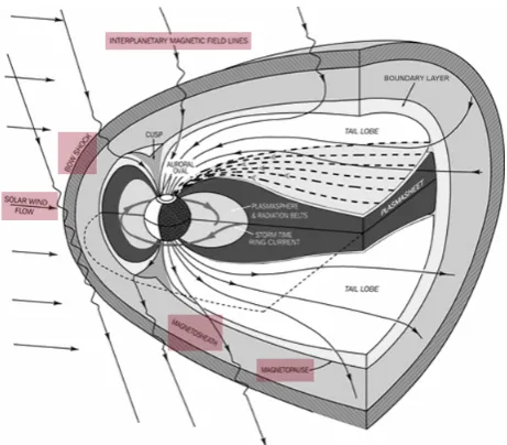
Fig. 1. 3-D picture of the Earth’s magnetosphere (adapted from http:
//pluto.space.swri.edu/IMAGE/glossary/magnetosphere.html). The plasma sheet and the tail lobe regions and cusps are distorted by the solar wind flow. The solar wind (exterior region) is outside the magnetopause. The boundary region is completed by the boundary layers, cusp, and the plasma sheet. The inner region contains tail lobe field lines that permeate the polar cap region.
magnetosphere regions widen like a funnel at radial distances 1Re≤r≤10 Re (Re is the Earth’s radius). At greater
dis-tances, e.g. at 10Re≤r≤15 Re, The solar wind blows the
two (northern and southern) high-latitude magnetosphere re-gions, flows around them and partly penetrates (see Fig. 1). The solar wind pressure becomes comparable to the Earth’s magnetic field pressure. The latter then cannot oppose the solar wind pressure, and the Earth’s magnetic field lines be-gin to be distorted. The solar wind direction, V0, however,
is still nearly perpendicular mainly to the (dayside) Earth’s magnetic fluxes. At greater distances, e.g. atr>20Re, the
Earth’s magnetic field lines are practically aligned to the so-lar wind velocity Vsw. At distances where the solar wind
ve-locity and the Earth’s magnetic field are practically parallel, the well-known Kelvin-Helmholtz instability and SW modes are easily excited. Another SW mode excitation mechanism exists, provided that the solar wind flow direction is nearly perpendicular to the Earth’s magnetic fluxes. This happens at distances where the angle between the solar wind veloc-ity and the magnetic field lines of the outer magnetosphere is close toπ/2, i.e. at distancesr≤15Re. The latter
mecha-nism of SW mode generation has been examined and mod-eled (Nenovski, 1996, 2003).
The high-latitude near-Earth magnetospheric regions (i.e. between distances 10Re<r<15Re)are assumed to be a flux tube of radius ρ1 (a cylindrical geometry). The existence
of a unified boundary region of free sizeρ1–ρ0, whereρ0
[image:3.595.313.544.64.266.2]284 P. Nenovski: Simulated and observed large-scale FACs This boundary region is characterized by plasma parameters,
whose content is different from those of the solar wind (de-fined as an open region of radiusρ>ρ1)and of the inner
re-gion of radiusρ<ρ0(that is the polar cap region). Thus, the magnetic flux tube (that interacts with the solar wind flow)
consists, on the one hand, of tail lobe field lines (the inner re-gion) of radiusρ<ρ0, and on the other hand, of mantle,
low-latitude boundary layer (LLBL), and the plasma sheet bound-ary regions. The latter are integrated in a unified boundbound-ary region lying betweenρ0andρ1. The SW mode field
distri-bution is expected to be localized at and around this bound-ary region (Nenovski, 2003). According to the magnetic flux conservation principle, all model results (e.g. FAC intensity, SW mode magnitude, etc.) obtained at distancer≈10–15Re
can be easily mapped to ionospheric heights. Roughly speak-ing, the situation of SW mode excitation by the solar wind at distancer≥10Reand their propagation properties (along the
magnetic field lines to the Earth, i.e. atr<10Re)might be
considered to be analogous to a propagation of electromag-netic signal along a transmission line. The point where this signal is forced is referred to as the source point. Condi-tions for generation of the SW modes of largest wavelengths, i.e. those of nearly zero-frequency domain, have been consid-ered (Nenovski, 1996). It is worth noting that even in zero-frequency limit, SW modes still propagate along the Earth’s magnetic field lines with the Alfv´en speedVA.
Equations that govern the SW mode FAC structure prop-agation are the MHD system and the ionospheric potential equation. The ionosphere is considered as a two-dimensional shell (Kelley, 1989; Raeder, 2003; Moretto et al., 2006): ∇ ·(6· ∇8)= −j||(rI)sin(I ), (1)
where8is the electric potential,6 is the ionospheric con-ductance tensor, I is the Earth’s magnetic field inclination angle,j||(rI)is the field-aligned current (FAC) intensity
cal-culated at ionospheric heights. The FAC intensity at iono-spheric heights j||(rI) is determined by transforming the
FAC intensity and distributionj||(rF AC)obtained from the
ideal MHD equations applied at source heightsrF AC≈10Re.
The geometry of the SW mode FAC system model is, how-ever, tied to the Earth’s magnetic dipole. Due to the Earth’s magnetic dipole rotation, the modeled “flux tube” axis cre-ates a variable angle with an eclipse and solar wind velocity V0. The solar wind and interplanetary magnetic field (IMF)
parameters thus have to be transformed to the Earth-centred (geocentric) solar magnetospheric coordinate system (GSM) (Russell, 1971). The latter has its x-axis from the Earth to the Sun. The y-axis is defined to be perpendicular to the Earth’s magnetic dipole, so that the x-z plane contains the dipole axis. The positive z-axis is chosen to be in the same sense as the northern magnetic pole. The northern magnetic pole that coincides with the flux tube orientation creates an angle2(tilt angle) with theZaxis. The IMF has two com-ponents,B0zandB0⊥, oriented along theZaxis and
perpen-dicular to it. It is worth noting that componentsB0zandB0⊥
22
Figure 2
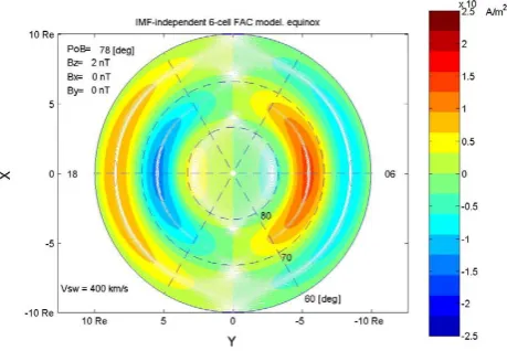
Fig. 2. This figure depicts a six-cell, large-scale FAC system (a
ground state) under equinox conditions where the IMF perpendicu-lar components,BxandBy, are taken to be equal to zero. The polar cap boundary (PoB) is taken at 78◦magnetic degrees and corre-sponds to an IMF equal to 2 nT. Note that this six-cell FAC system can also exist under zero IMFBz conditions. The FAC intensity is evaluated at ionospheric heights (given in polar coordinate sys-tem), taking into account the magnetic flux conservation principle. The source region is assumed at a radial distancer equal to 10Re (shown by X0Y coordinates). Red color and positive FAC intensity values correspond to inward FAC flowing toward the ionosphere, blue color and negative FAC values – to outward FAC flowing away from the ionosphere. The FAC intensity distribution possesses a maximum around 1µA/m2.
differ from conventional IMFBx,By,Bzcomponents in the
Geocentric Solar Ecliptic (GSE) coordinate system.
In the zero-frequency approximation a stream function (potential)ϕand vector magnetic field potential A of the SW modes are well introduced. Then
v=rotϕ+V0andb=rotA,
where V0≡Vsw(2) is the solar wind flow mapped on the
chosen geocentric GSM coordinate system. It depends on 2. The solar wind speed, Vsw and the IMF components are
assumed to be homogeneous.
The following basic equation of the velocity stream func-tionϕhas been derived (Nenovski, 1996):
[ϕ−V0y, 1ϕ]=R−2[D(ϕ−V0y), P]+
R−1[M(ϕ−V0y), 1M(ϕ−V0y)]
, (2)
where R and P are plasma density and pressure, respec-tively. Magnetic field vector potential A and pressureP are expressed by
A=m(ϕ−V0y)+γ , P=d(ϕ−V0y)+δ, (3)
[image:4.595.313.543.68.227.2]P. Nenovski: Simulated and observed large-scale FACs 285 the following boundary conditions: i) the continuity of the
potentials (velocity and magnetic field) through interfaces ρ=ρ0,1; ii) a constancy of the potentials along
circumfer-encesρ=ρ0,1; and iii) the finiteness of the SW mode energy
at infinity,ρ→∞. The latter means that we have to meet the condition for zero magnitude of SW mode potentials at infi-nite. Vector magnetic field potentialAis related to the SW velocity stream functionϕ (3). Coefficientm(that relates the magnetic field and velocity potentials) is thus equal toB0/VA
(Wal´en relation), whereB0is the Earth’s magnetic field
mag-nitude,VAis the Alfv´en velocity. The FACs distribution and
propagation dynamics are described by relation j||=−µ−011A.
The model yields a FAC intensity and distribution that de-pends directly on the solar wind and magnetosphere parame-ters. In general, the SW mode magnetic field and the FAC in-tensity in all FAC cells are controlled by the density/pressure gradient scale λe at the Earth’s magnetopause (Nenovski,
2003), defined by:
λe≡(R0−1dR0/dx)−1=P0−1dP0/dx)−1.
Gradient ∇P0 is equal to 1/2 RswV0E2 /ρ1, where Rsw and V0E are the solar wind density and the magnitude of the
Earth’s orbital velocity, respectively. The FAC intensity dis-tribution, being connected to the plasma pressure gradient scaleλe, will be controlled by solar wind velocity V0, the
IMF magnitude and orientation, As expected, the large-scale FAC intensity dynamics depends also on internal parameters: the Earth’s magnetic field magnitude (at the magnetopause), B0; the plasma density distribution,R (entering through the
Alfv´en velocityVA); the tilt angle,2and characteristic scale, λF AC, that is inversely proportional to the boundary region
cross sizeρ1-ρ0, i.e. λFAC∝(ρ1−ρ0)−1.
In previous analyses (Nenovski, 1996, 2003), the IMF mag-nitude and orientation have been coupled with the solar wind velocity magnitude V0. The large-scale FAC intensity is
thus a function of the IMFBx component, i.e. the
previ-ous FAC model concerns an IMF-dependent FAC solutions. In the present study, all the IMF components, Bx, By and Bz, are taken into account, and the IMF and solar wind
ve-locity potentials are decoupled. Both IMFBxandByeffects
are treated here and represent a particular solution of the SW mode FAC model. The large-scale FAC structure is again determined by general dispersion equations derived for arbi-trary IMFBx andBz and zero IMFBy. Due to the Earth’s
magnetic field dipole axis orientation, the projection of the IMFBz component onto the equatorial plane of the Earth’s
magnetic field will additionally change the FAC current dis-tribution.
Without quoting all mathematical procedures, the follow-ing dispersion equation that determines all the structural pa-rameters of nonlinear (NL) SW modes and the associated
FACs system under assumed geometry is derived: k2r12[−Y1(kρ1)J1(kρ0)+Y1(kρ0)J1(kρ1)]K2(qeρ1)/
K1(qeρ1)+qekρ12[Y1(kρ0)J2(kρ1)−Y2(kρ1)J1(kρ0)]
=2qeρ0/π,
(4)
qeρ1[−Y2(kρ0)J2(kρ1)+Y2(kρ1)J2(kρ0)]
+kρ1[Y1(kρ1)J2(kρ0)−Y2(kρ0)J1(kρ1)]K2(qeρ1)/
K1(qeρ1)=2qeρ0I2(qiρ0)/π qiρ1I1(qiρ0).
HereJnandYn are Bessel functions,InandKn (n=0,1) are
modified Bessel functions; k and qi, are structural
param-eters of the system that have to be found; radiusρ0 andρ1
are free (input) parameters;qe2=−βe/V0x≡dR−sw2(dP/dy)/V0.
Normalized by radius (ρ1)structural parameters k and qi,
(i.e. quantities qiρ0 and kρ1) have to be determined from
(4). The SW mode wave number,k, determines the number of FAC structures in the boundary regionρ0<ρ<ρ1; wave
numberqi characterizes the SW field structure in the inner
regionρ<ρ0. Dimensionless quantityqeρ1=
√
(βρ21/V0)is
equal toV0E/V0.
The FAC intensity, j|| can be derived from the
mag-netic field potential A (1) by the relationship j||=−µ−01
1A≡−µ−01B01ϕ/VA. It can be found that
j||,g∝ V0(2)(Rb)1/2/ρ1λ2F AC(IMFBz), (5)
whereRbis the plasma density in the boundary region, and
scaleλFAC is the IMFBz dependent parameter. Note that
FAC density j||,g is inversely proportional to the squared
scaleλFAC. In the polar cap region,λFAC,pc≡1/qi, in Region
1 and Region 2, FAC scaleλFAC,R1+R2≡1/k. Under negative
IMFBz, the scale of the polar cap radiusρ0 increases and
the size ρ1−ρ0 decreases, hence λFAC,pc decreases, while
the scaleλFAC,R1+R2(∼(ρ1−ρ0)−1)increases. Under
posi-tive IMFBzthe polar cap radius,ρ0decreases and the size ρ1−ρ0 increases, hence λFAC,pc increases, while the scale λFAC,R1+R2(∼(ρ1−ρ0)−1)decreases. The IMFBx andBy
components introduce FACs that are proportional to
j||,Bx(By)=.Bx(Byρ/λFAC(IMFBz))(Rm)1/2/ρ1λ2FAC(IMFBz), (6) As follows from Eq. (6) the FAC induced by the IMF By
component isρ/λFAC,R1+R2 times the FAC induced by the
IMFBx component. Compared to Eq. (5) the IMFBy FAC
magnitude is VA,bBy/V0B0 times the ground-state FAC
in-tensity. Let us make some estimate of the ratioVA,bBy/V0B0.
286 P. Nenovski: Simulated and observed large-scale FACs (Runov et al., 20071). In the high-altitude polar cusp the
Alfv´en velocity is 200–800 km/s (Grison et al., 2005). In the high-latitude boundary layer (HLBL) the local Alfv´en velocity is about 350 km/s at distance 10Re (Nykyri et al.,
2006). The measured Alfv´en speed in different boundary lay-ers, like LLBL, HLBL, and the high-altitude cusp thus proves to be mostly in the interval 200–800 km/s. The plasma den-sity in the polar cap region varies between 0.2–1 part/cm3, in the boundary region (LLBL), is by an order higher (1– 10 part/cm3) (Nykyri et al., 2006). In the inner/polar cap region the Alfv´en velocity is taken to be proportional to (Rm/Rpc)1/2VA,b, whereRbandRpc are the plasma
densi-ties in the boundary region and in the polar cap, respectively. In our large-scale FAC simulation the Alfv´en velocity,VA.b,
in the boundary region, is taken to be equal to 400 km/s. For convenience, theRm/Rpc ratio is assumed to be equal to 20.
The other quantities, IMFBycomponent, solar wind speed, V0 and magnetopause magnetic field, B0 are, in principle,
known. TakingVA andV0to be equal to 400 km/s and the
magnetic fieldB0at the magnetopause to be of the order of
100 nT, the ratioVA,bBy/V0B0thus rarely exceeds a value of
0.1.
FAC simulations yield that the IMFBxcomponent
contri-bution to the large-scale FAC intensity is practically by an order less than the IMFBy component contribution. The
IMF By component contribution (proportional to the
ra-tioρ/λFAC,R1+R2>1) may, however, constitute tens or even
more percents of the large-scale FAC ground-state magni-tude.
The SW mode FAC system structure depends on external parameters: qe,V0, IMF components, Bx, By andBz, and
internal parameters:B0, plasma density distributionRm, and
radiusρ0,1. Radius ρ0 and radius ρ1 are free parameters
of the proposed SW mode FAC model. Actually, they have to be related to the polar cap boundary and the lowest lati-tude of the disturbed magnetic field lines. Radius,ρ0(1) is
thus closely connected with the sign and magnitude of the IMFBzcomponent. Following experimental evidences,
un-der positive IMFBzconditions, the polar cap boundary (that
corresponds to radiusρ0)is close to the 80◦magnetic
lati-tude; under negative IMFBzthe polar cap boundary is∼at
75◦and lower. The external radiusρ1also depends on the
solar wind and IMF parameters. Radiusρ1and plasma
den-sity variations in the boundary regionρ0<ρ<ρ1have to also
be treated as a function of the previous state of the magne-tosphere and thus these parameters reflect the dynamic his-tory of the Earth’s magnetosphere. Their actual magnitudes seem to be connected with the inner magnetosphere condi-tions, i.e. they are inertial ones. In our analysis we assume that radiusρ1 and plasma density distributionRm are
con-stants. For convenience, radiusρ1is assumed to correspond
to 60◦(magnetic latitude).
Large-scale FAC system – a ground state
A ground state of the large-scale FAC system, consisting of six cells, can be recognized if one considers all the IMF com-ponents to be nearly equal to zero. In our FAC calculations the magnitude of the Earth’s magnetic field at the magne-topauseB0 is taken to be equal to 120 nT, the solar
wind-magnetosphere interaction occurs at radial distancer=10Re,
the solar wind velocity V0 varies, or is equal to 400 km/s,
the tilt angle2is assumed for summer, equinox and winter conditions. Actually, the Earth’s magnetic field at the mag-netopauseB0is dependent on solar wind pressure variations,
thus the solar wind velocity and theB0magnitude are in fact
interrelated. When the solar wind velocity increases,B0also
increases. For comparison with experimental data obtained mainly from low-altitude satellites, a map of the FAC inten-sity along the magnetic field tube to ionospheric heights is required. Due to the flux conversion (B.S = const) the FAC intensity converges, as well. The FAC intensity depends on radial distance r (from the Earth’s surface) as (rFAC/rI)3,
whererFACis the radial distance of the FAC source andrIis
the ionosphere shell distance (rI∼=Re). Thus, at ionosphere
heights (rI∼=Re)the FAC intensity will increase roughly by
three orders compared to its density at the FAC source dis-tance (rFAC∼=10Re). In Fig. 2 the FAC intensity is evaluated
at ionospheric heights, taking into account the magnetic flux conservation principle. The polar cap boundary is taken to be equal at 78◦ magnetic degrees and corresponds to IMF Bzequal to 2 nT. The IMFBxandBycomponents are set to
zero.
The six-cell FAC ground state given in Fig. 2 depicts the main experimental features of the large-scale FAC structure satellite observations. FAC intensity distribution possesses maxima and minima close to the central dawn-dusk line, and the absolute values of the Region 1 FAC intensity exceed the absolute values of the Region 2 FAC intensity. The FAC in-tensity distribution possesses a maximum that is below but close to 1µA/m2. Note that the SW mode FAC model yields a quantitative relationship between the FAC intensity and the solar wind velocityV0and the boundary plasma densityRb.
According to the model (Eq. 5) the FAC density is propor-tional to solar wind velocityV0and boundary plasma density
(Rb)1/2.
The IMF influence on the large-scale FAC system is exam-ined further. The six-cell FAC ground state still exists under various IMF conditions. Considering the IMF By
compo-nent to be equal to zero (while IMFBx andBzcomponents
are variable), the zero-frequency SW mode FAC model again yields an existence of a six-cell FAC structure, as was previ-ously discovered (Nenovski, 2003). The relevant IMF com-ponents are easily transformed from the GSE to GSM coordi-nate system by a simple rotation about the x-axis. This means that the IMF componentsBx(By) are influenced by the IMF Bz component under summer/winter (equinox) conditions.
P. Nenovski: Simulated and observed large-scale FACs 287 that depends on the IMFBz component only. Three values
of the IMFBz component are chosen: Bz=2 nT,Bz=10 nT,
andBz=−10 nT. For IMFBz=2 nT the polar cap boundary is
taken to be equal to 78 degrees, forBz=10 nT, this boundary
is 82 degrees, and forBz=−10 nT, the polar cap boundary is
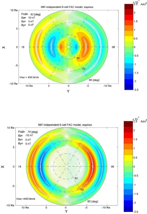
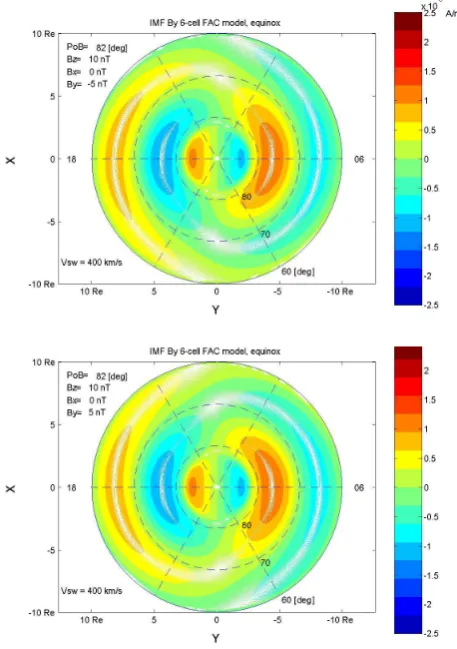
74 degrees. Figure 3a, b depicts a six-cell FAC system where the IMFByis set to zero under equinox conditions.
The FAC structure demonstrates variations of the FAC density in the polar cap depending on the IMFBzcomponent
magnitudes. When the IMFBzbecomes negative, the FAC
intensity in the polar cap decreases and under strong nega-tive IMFBzconditions (IMFBz equals to−10 nT) the
ini-tial six-cell FAC structure practically evolves into a four-cell FAC structure that occupies the boundary region (ρ0≤ρ≤ρ1)
only. Inversely, when the IMFBz is positive the 6-cell FAC
structure emerges clearly and the polar cap FAC (dipole) structure is of high intensity. Region 1 and Region 2 FAC systems thus co-exist.
In Fig. 3a, b the boundary plasma density is chosen to be invariable. Note that the induced FAC intensity variations are a function not only of the boundary region size, but also of the plasma density variations in the boundary regions under a different sign of the IMFBz.
IMFByeffects on the large-scale FAC system
Further, in our analysis we will be concerned with the effects of IMFBy, as well as the possible changes caused by the
negative/positive IMFBzcomponent on the FAC system.
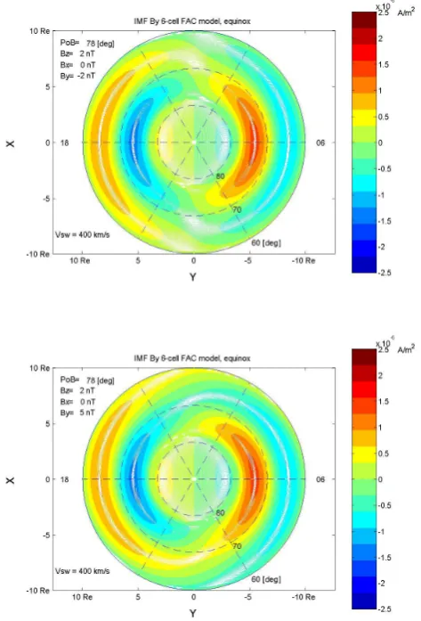
Examples of large-scale FAC structures as a solution for the Eq. (2) are given in Fig. 4a–c. Figures 4a–c illustrate large-scale FAC structure as influenced under negative, zero and positive IMFBy. The IMFBzandBxare taken to be
pos-itive and equal to 2 nT. The inner radiusρ0is chosen to be at
78 degrees (that corresponds to northward IMF conditions), the outer radiusρ1corresponds to 60 degrees. The other
pa-rameters are: the solar wind velocity is 400 km/s, the bound-ary density is 10 particles/cm3, the number density in the tail lobe is 20 times less. Figures 4a–c reveal the effects as ex-pected from the DPY current system: during positive IMFBy
the Region 1 FAC system from the dawn sector is extended across the noon sector. This FAC attaches the dusk part of the FAC system in the polar cap. On the other hand, the Region 1 FAC system from the dusk sector (of inverse polarity) con-tinues into the Region 2 FAC system from the dawn sector. This FAC structure modification clearly emerges only under stronger IMFBymagnitudes (when the IMFBymodule
ex-ceeds 2 nT). It seems that the six-cell FAC structure would evolve into two FAC “spirals” of inverse polarity where both spirals start from the polar cap regions. If the IMFBysign
reverses, the sense of the FAC “spirals” also reverses. In the midnight sector the dawn (dusk) Region 1 FAC structure goes continuously to the dusk (dawn) Region 2 FAC cell.
Under equinox conditions the FAC intensities from both hemispheres are expected to be equal to each other. The
23
Figure 3a and b
Fig. 3. FAC density variations in the polar cap (the dipole FAC
structure), depending on the IMFBz component magnitudes, are illustrated. This figure depicts a six-cell, large-scale FAC system under equinox conditions where the IMF perpendicular component, By, is assumed to be equal to zero. The coordinates are the same as in Fig. 2. Under negative IMFBzconditions (IMFBzequals to
−10 nT) the initial six-cell FAC structure practically evolves into a four-cell FAC structure that occupies latitudes 60◦–74◦magnetic degrees only. Inversely, when the IMF Bz is positive (IMFBz equals to 10 nT) the six-cell FAC structure clearly emerges where the polar cap (dipole) FAC structure is of high intensity.
[image:7.595.310.544.65.406.2]288 P. Nenovski: Simulated and observed large-scale FACs
24
Figure 4a
Fig. 4a. Illustrate how a negative/positive IMFBycomponent in-fluences the SW mode FAC structure. During positive IMFBy, the Region 1 system from the dawn sector is extended across the noon sector. On the other hand, the Region 1 system from the dusk sector (of inverse polarity) continues into the Region 2 system from the dawn sector. When the IMFBymodule well exceeds 2 nT, the six-cell FAC structure evolve into two FAC “spirals” of inverse polarity. When the IMFBycomponent reverses its sign, the sense of the FAC “spirals” also reverses. In the midnight sector the dawn (dusk) Re-gion 1 structure goes continuously to the dusk (dawn) ReRe-gion 2 cell. The IMFBzcomponent is set to−10, 2 and 10 nT. Figure 4b is for IMFBz=−10 nT, and 4c – for IMFBz=10 nT.
high-latitude magnetic field lines create with the solar wind direction an angle well below angleπ/2; the solar wind ve-locity thus may not encounter effectively the high-latitude near the Earth’s magnetic flux tube. A decrease in the FAC intensity, additional to factor cos(2) thus will emerge. Note only the nonzero projection of the solar wind velocity vec-tor on the plane perpendicular to the Earth’s magnetic fluxes is responsible for the large-scale FAC structure generation. Qualitatively, the FAC intensity difference between summer and winter conditions may be assumed to be proportional to the ratio of the high-latitude Earth’s magnetic flux volume
[image:8.595.312.545.64.416.2]25
[image:8.595.49.286.66.415.2]Figure 4b
Fig. 4b. Continued.
encountered by the solar wind flow. The two effects result in a FAC intensity difference between summer and winter. In comparison to the equinox conditions the FAC intensity for summer becomes 1.6 times greater. Under winter conditions the FAC intensity is, however, approximately three times less than in equinox. Figure 5a, b characterizes the six-cell FAC structure under summer and winter conditions.
The SW mode FAC model also reveals some difference that depends on the magnitude of the IMF Bz component.
This difference comes from the different sign of the IMFBz
projection on the equatorial plane of the Earth’s magnetic field dipole axis. Hence, the contribution of the IMFBy
ef-fect, i.e. the IMFByFAC intensity may be different.
3 Comparison with experimental data
The modelled FAC intensity j|| at ionosphere heights
P. Nenovski: Simulated and observed large-scale FACs 289
26
[image:9.595.314.541.66.395.2]Figure 4c
Fig. 4c. Continued.
conditions 2−≤Kp≤4+the Region 1 FAC maximum inten-sity amplitude was 2.0(1.3)µA/m2 and the Region 2 FAC maximum intensity amplitude was 1.0(0.6)µA/m2) at the morning (evening) sectors (Iijima and Potemra, 1978). The first statistical picture of FACs contains intense FAC struc-tures (of∼1.0µA/m2)in the nightside sector, not predicted in our zero-frequency MHD surface mode model. This is be-cause Iijima and Potemra’s FAC picture integrates FAC struc-ture intensifications during dynamic processes, like magne-tospheric (sub)storms released under negative IMFBz
con-ditions, where merging/reconnection-like processes occupy the evening-midnight sector of the polar ionosphere.
Recently, precise magnetic field measurements on board two satellites, Magsat and Oersted, have demonstrated new properties in the physics of steady-state FAC systems. Using data from Magsat and Oersted high-precision magnetic mea-surements the satellite orbits have been sorted on the basis of strict criteria to ensure steady IMF and solar wind
con-ditions at the time of the polar pass (Stauning, 2003).
Ex-perimental evidences and results have been summarized by Stauning (2003). Thus, the proposed large-scale FAC struc-ture model could be tested on the observed FAC systems un-der various IMF conditions – positive and negative IMFBz,
27
Figure 5a and 5b
Fig. 5. Figure 5a, b characterize the six-cell FAC structure under
summer and winter conditions. In comparison to equinox condi-tions (not shown) the FAC intensity in summer becomes 1.6 times greater. Under winter conditions the FAC intensity is, however, ap-proximately three times less than in equinox.
dominant IMF By component, summer/winter, or equinox,
etc. The NBZ FAC intensity over the northern polar cap attains a magnitude of 1µA/m2and more when there is the summer season and the IMFBzcomponent is within
inequal-ities: 10 nT<IMFBz<20 nT (Stauning, 2002). Our results on
[image:9.595.50.279.68.393.2]290 P. Nenovski: Simulated and observed large-scale FACs them has to be enhanced. Thus, both magnetic flux and
re-spective FAC density on the noon part of the polar cap should be more enlarged compared to that on the nightside.
Differences in the FAC intensity due to the season and the IMFBz sign are examined by Stauning (2003). When the
IMFBy component is close to zero (−2 nT<IMFBy<2 nT)
and the IMFBzcomponent is variable, the FAC density
be-comes its maximum either in the polar cap (the IMFBz is
then positive (>5 nT), or in the Region 1 FAC system (the IMFBz is then negative,−10 nT<IMFBz<−5 nT). In the
first case the polar boundary of the Region 1 FAC system is at 80◦magnetic latitude, in the second case (of negative IMF Bz)the Region 1/2 FAC systems occupy a belt of some 15
degrees, i.e. between 60◦–75◦magnetic latitude. By an exact choice of the inner radiusρ0(the polar cap boundary), the
proposed FAC system model (Figs. 2–5) reconciles the main features of the observed FAC distribution (under equinox and summer/winter conditions) and their maxima around the cen-tral dawn-dusk line.
The IMFByinfluence on the FAC system has been also
ex-amined. Stauning (2003) has displayed the FAC structure un-der equinox and negative IMFBz (−5 nT<IMFBz<−2 nT)
conditions. Two solar wind velocity regimes are considered: 200<V0<400 km/s and 400<V0<900 km/s. The FAC
densi-ties have their extrema in the Region 1 FAC system and again at the dawn-dusk central line, and are proportional to the so-lar wind velocity magnitude. The FAC structure is practically a four-cell one. A single downward/upward polar cap FAC cell centred at noon and at 80◦, or at 80◦–85◦magnetic lat-itudes under positive/negative IMFBy, may additionally be
recognised. Another polar cap FAC cell of inverse polarity, however, cannot be identified clearly. Having in mind our findings of the emergence of spiral-like FAC structures un-der dominant IMFBy, such an asymmetry in the polar cap
FAC structure seems not to have experimental verification. When the interplanetary magnetic field (IMF) was either near zero, or different from zero (with IMFBz>0 and IMF Bz<0), a persistent pair of FACs of inverse polarity flowing
poleward of the Region 1 FAC system and placed in the cen-tral area of both the southern and northern polar caps has been discovered (Papitashvili et al., 2001, 2002; Weimer, 2001b; Stauning, 2002). The distribution of these currents under IMF orientation resembles the dayside NBZ system, with the downward/upward currents at post-noon/pre-noon hours. Hence, the polar cap FAC system polarity is opposite to that of the Region 1 FAC system.
Let us quantitatively compare the SW mode FAC system to empirical large-scale FAC models based on Oersted and Magsat satellite data. A steady-state FAC distribution for a different IMF clock angle has been derived (Papitashvili et al., 2001, 2002). Analyzing the IMFBy=0 case, the FAC
intensity usually is maximum in the Region 1 FAC system, except when the IMF Bz>0 and in the southern (summer)
hemisphere case. The FAC intensity maximum in the Re-gion 1 FAC system in the Southern (Northern) Hemisphere
varies from +0.56(0.35) to−0.51(0.29)µA/m2under south-ward IMFBzconditions in the morning (sign +) and evening
(–) sectors. Signs +/−refer to the downward/upward FACs in the morning/evening sectors. Under northward IMFBz
conditions the FAC intensity in Region 1 are weaker: from 0.07 to−0.15µA/m2in the Northern (winter) Hemisphere. Surprisingly, the upward FAC intensity in the Southern (sum-mer) Hemisphere has its absolute maximum in the polar cap: −0.3µA/m2. The downward FAC intensity, however, per-sists in the Region 1 FAC system: +0.15µA/m2. Satellite observations have revealed a strong control of the IMFBy
component on the polar cap FAC intensity in the summer hemisphere. The average magnitude of Region 1 FAC varies between 0.1 and 0.56µA/m2.
An evaluation of the total FAC flowing in and out of the ionosphere can be performed choosing all FAC cells of one polarity and integrating the FAC intensity. As a rough esti-mate, the total FAC of one polarity (depending on the season conditions) amounts to 105–106A, depending on solar wind, IMF and seasons conditions. The result is in keeping with experimental evidences.
The negative/positive IMFBz is suggestive for different
plasma dynamics and densities in the boundary regions; this results in a different amount of available FAC carriers within them. Accordingly, the SW mode FAC model yields a FAC intensity distribution depending on the boundary/polar cap density ratio. The SW mode FAC model is also sensitive to the solar wind parameter variations. The Papitashvili et al.’s (2002) result based on Oersted observations represents an av-erage FAC picture depending on the IMF clock angle and is irrespective of the solar wind velocity variations. Neverthe-less, the six-cell FAC system (one pair FAC structure in the polar cap and two pairs of FACs in the boundary (auroral) re-gions) predicted by the SW mode FAC model, may find their counterparts in the Oersted satellite observations. The FAC intensities calculated from both the SW mode FAC model and Oersted data are of comparable magnitudes.
The SW mode FAC model thus yields qualitatively and quantitatively a good correspondence with experimental re-sults for reasonable values of the solar wind velocity and IMF parameters. The correspondence consists of: (i) two pairs of FAC structures of inverse polarity that emerge within the boundary region (ρ0<ρ<ρ1). They may be interpreted as
Region 1 and Region 2 FAC structures observed in the au-roral region; (ii) a pair of FAC structures of inverse polar-ity in the inner region (ρ<ρ0). This polar cap FAC
struc-ture exists under the arbitrary sign of the IMF Bz
compo-nent but its intensity is much higher under northward IMF Bz. The latter may be considered as tail-lobe FACs; and
P. Nenovski: Simulated and observed large-scale FACs 291 desirable, especially for the cases with a positive IMF Bz
component. Further, the effects of the plasma density change in the boundary region (ρ0<ρ<ρ1)during positive/negative
IMFBzon large-scale FAC distribution need to be precisely
estimated.
In conclusion, a dipole-like (two cells of inverse polar-ity) FAC system in the inner regionρ<ρ0(polar cap, or tail
lobe) and four (two pairs) FAC cells of inverse polarity (that encircle the dipole FACs), localized in the boundary region ρ0<ρ<ρ1, can co-exist (Nenovski, 2003). It is worth
not-ing that in the boundary region solutions of Eq. (4) with a lower number of FAC cells (less than 4) cannot be found, i.e. at least 4-cell FACs (Region 1 and Region 2 FACs) in the boundary region co-exist with a pair of (dipole) FACs in the polar cap. These crescent-like FAC regions (belts) encircle azimuthally the dipole/central FAC structure. The complete FAC system is flowing (along the magnetic field lines) to-ward the Earth. The FAC intensities in all regions have their maxima/minima around the line perpendicular to the solar wind flow (V0), going through the locus of the circle of
in-teraction.
The results derived from the SW mode FAC model sug-gest that a common nonlinear MHD mechanism of the solar wind-magnetosphere interaction can only support a six-cell large-scale FAC structure. This six-cell structure exists even under zero IMF conditions. An inclusion of IMF components reveals the principal features inherent either to the NBZ FAC system that exists under positive IMFBz, or to the Region 1
and Region 2 FAC system under stable negative IMFBz
con-ditions. An inclusion of the IMFBy component produces
a Region 1 FAC extension over the noon sector that corre-sponds to the DPY system. Obviously, the proposed large-scale SW mode FAC structure is consistent with processes (viscous and/or merging ones) that have been suggested in previous FAC models.
The above general conclusions need some further remarks. Even in steady-state conditions the primary six-cell FAC sys-tem may be easily destroyed toward the Earth’s ionosphere. First, due to the Earth’s magnetic field line conversion, the FAC intensity grows and under appropriate conditions can easily exceed a magnitude of 10−6A/m2. Such FAC in-tensity magnitudes may be sufficient for plasma instability outbursts. An instability of large-scale FAC may result in FAC structure changes also, e.g. the appearance of multi-ple FAC structures of a smaller size. As a result, the inten-sity of the FAC structures of medium size will exceed those of the large-scale ones. Second, the FAC Joule dissipation rate in the ionosphere will be qualitatively and quantitatively different with and without multiple FAC structures. Satel-lite observations of FAC structures and the associated con-vection electric field in the polar ionosphere have already confirmed the existence of more intense multiple FAC struc-tures and stronger convection electric fields (e.g. Ohtani et al, 1994; Eriksson et al., 2002). Existing convection electric field models (e.g. Weimer, 2001a, b; Papitashvili and Rich,
2002) have lacked the ability to simulate more intense struc-tures of medium scales, i.e. those of several hundreds of km, observed, say, by the Astrid-2 satellite.
An emergence of structures of medium scales a in the large-scale FACs regions and in the global convection elec-tric field in the polar/polar cap ionosphere may be a direct consequence of the FAC pattern instability treated by Nen-ovski et al. (2003). Without quoting the formalism of the structural instability that follows from the FAC intensity in-crease toward the ionosphere, the FAC pattern formation be-gins at
j||,crita ≥0.2(vT/vT o)[A/m], (7)
wherevT ois the “thermal” velocity of the FAC carriers that
corresponds to plasma temperatureT0 of 0.1 eV. The FAC threshold value intensity magnitude increases with the
“ther-mal” velocityvT of the FAC carriers. The obtained threshold
value (7) can be expressed by the associated convection elec-tric field E that is mapped along the magnetic field lines to the ionosphere heights. Depending on the ionospheric Pedersen and Hall conductances, the threshold values,Et hreshwill be
of different magnitude. In its simplest form (homogeneous Pedersen and Hall conductances) the following relationship betweenEthreshandj||,crit(m, n) can be derived from Eq. (1):
Ethresh=j||,crit(m, n)/6p. (8)
The ionospheric conductances are greatest in the auroral re-gions compared with those in the polar cap. Hence, multiple FAC structures can be easily excited within the auroral oval. Taking the Pedesen conductance6pvalues of 10 S (a modest
value) we found that a convective electric field magnitude of 20 mV/m can initiate multiple FAC/electric field structures. Such values are often detected on board the Astrid satellite (Eriksson et al., 2002). Note that the existence of the elec-tric fields of magnitude 20 mV/m, however, does not neces-sarily involve the formation of multiple FAC structures. In terms of the Pedersen current, the necessary condition is that
Ethresh6p should exceed the critical value of 0.2 A/m (see
Eq. 7).
4 Consequences and conclusion
The principal issues that follows from the suggested SW mode FAC model are i) the large-scale FAC intensity and dis-tribution in the polar ionosphere can be quantified provided that the solar wind, IMF and magnetospheric (polar cap/ and inner plasma sheet boundaries) parameters are known. Using these parameters as input parameters large-scale FAC charac-teristics in the polar regions can be derived and compared to available observational data.
The existence is predicted for ground-based six-cell FAC based on a nonlinear surface wave excitation mechanism at
292 P. Nenovski: Simulated and observed large-scale FACs structure exists irrespective of the sign of the IMFBz
com-ponent. The main peculiarity of this mechanism is the co-existence of two pairs of FAC structures of opposite polarity (that correspond to Region 1 and Region 2 FAC), co-existing with a pair (dipole) of FAC structures over the polar cap. The SW concept of large-scale FACs also provides reason-able magnitudes of the morning and dusk part of the large-scale Region 1 and 2 FACs, depending quantitatively on the solar wind and IMF parameters, the Earth’s dipole axis ori-entation, etc.
Comparison with high-precision magnetic observations from Magsat and Oersted satellites gives a good correspon-dence between the observed FAC structures under steady-state conditions (Stauning, 2002, 2003) and those modelled by the zero-frequency SW mode excitation mechanism.
Main factors that can distort the predicted six-cell FAC structure are i) the indispensable intensification of the large-scale FAC density and ii) the transition from high to lowβ plasma conditions along their propagation direction. Both factors could facilitate FAC structures of different scales at appropriate FAC intensity threshold values. FAC pattern for-mation processes expected at ionosphere heights could be the most favourable mechanism of periodic FAC structures ob-served in high-latitude regions.
Large-scale FAC structure and associated FAC pattern for-mation processes being controlled by the solar wind and IMF conditions generate an associated electric potential distribu-tion in the polar ionosphere regions and determine the Joule dissipation rate.
Acknowledgements. The author would like to express his thanks to J. Watermann for providing publications and proceeding mate-rials from DMI, Copenhagen on magnetometric measurements on Magsat and Oersted satellites. The author also thank to both refer-ees for their valuable criticism and comments that help to improve all issues from this study. This study was partly supported by the NSF Bulgarian Grant ES-1502/2005.
Topical Editor W. Kofman thanks J. Watermann and V. Pap-itashvili for their help in evaluating this paper. He also thanks F. Lefeuvre for his help in evaluating this paper.
References
Akasofu, S.-I., Ahn, B.-H., and Kisabeth, J.: Distribution of field-aligned currents and expected magnetic field perturbations re-sulting from auroral currents along circular orbits of satellites, J. Geophys. Res., 85, 6883–6887, 1980.
Boyle, C. B., Reiff, P. H., and Hairson, M. R.: Empirical polar cap potentials, J. Geophys. Res., 102, 111–125, 1997.
Christiansen, F., Papitashvili, V. O., and Neubert, T.: Seasonal variations of high-latitude field-aligned currents systems in-ferred from Oested and Magsat observations, J. Geophsy. Res., 107(A2), 1029, doi:10.1029/2001JA900104, 2002.
Eriksson, S., Blomberg, L. G., and Weimer, D. R.: Comparing a spherical harmonic model of the global electric field distribution with Astrid-2 observations, J. Geophys. Res., 107(A11), 1391, doi:10.1029/2002JA009313, 2002.
Erlandson, R.E., Zanetti, L. J., Potemra, T. A., Bythrow, P. F., and Lundin, R.: IMFBydependence of region 1 Birkeland currents near noon, J. Geophys. Res., 9, 9804–9814, 1988.
Friis-Christensen, E., Kamide, Y, Richmond, A. D., and Matsushita, S.: Interplanetary magnetic field control of high-latitude electric fields and currents determined from Greenland magnetosmeter data, J. Geophys. Res., 90, 1325–1338, 1985.
Grigorenko, E. E., Sauvaud, J.-A., and Zelenyi, L. M.: Spatial-temporal characteristics of the beamlets in the plasmasheet boundary layer of magnetotail, J. Geophys. Res., 112, AO5218, doi:10.1029/2006JA011986, 2007.
Grison, B., Sahraoui, F., Lavraud, B., Chust, T., Cornilleau-Wehrlin, N., Reme, H., Balogh, A., and Andre, M.: wave particle interactions in the high-altitude polar cusp: a Cluster case study, Ann Geophys., 23, 3699–3713, 2005.
Iijima, T. and Potemra, T.: The amplitude distribution of field-aloigned currents at northern high latitudes observed by Triad, J. Geophys. Res., 83, 1109–1114, 1976a.
Iijima, T. and Potemra, T.: Field-aligned currents in the dayside cusp observed by Triad, J. Geophys. Res., 81, p. 5971, 1976b. Iijima, T. and Potemra, T.A.: Large-scale characteristics of
field-aligned currents associated with substorms, J. Geophys. Res., 83, 599–615, 1978.
Iijima, T., Potemra, T. A., Zanetti, L. J., and Bythrow, P. F.: Large-scale BIrkeland currents and the dayside polar region during strongly northward IMF: A new Birkeland current system, J. Geophys. Res., 89, p. 7441, 1984.
Kan, J. R. and Lee, L. C.: Energy coupling function and solar wind-magnetosphere dynamo, Geophys. Res. Lett., 6, 577–600, 1979. Kelley, M. C.: The Earth’s Ionosphere. Academic Press, New York,
1989.
Lu, G., Lyons, L. R., Reiff, P. H., Denig, W. F., de la Beaujardi´ere, O., Kroehl, H. W., Newell, P. T., Rich, F. J., Opgenoorth, H., Persson, M. A. L., Ruohoniemi, J. M., Friis-Christensen, E., Tomlinson, L., Morris, R., Burns, G., and McEwin, A.: Char-acteristics of ionospheric convection and field-aligned current in the dayside cusp region, J. Geophys. Res., 100(A7), 11 845– 11 862, 1995.
Moretto, T., Vennerstrom, S., Olsen, N., Rastatter, L., and Raeder, J.: Using global magnetospheric models for simulation and inter-pretation of SWARM external field measurements, Earth Planets Space, 58, 439–449, 2006.
Ohtani, S., Zanetti, L. J., Potemra, T. A., Baker, K. B., Ruohoniemi, J. M., and Lui, A. T. Y.: Periodic longitudinal structure of field-aligned currents in the dawn sector: large-scale meandering of an auroral electroject, Geophys. Res. Lett., 21, 1879–1882, 1994. Ogino, T., Walker, R. J., and Ashour-Abdalla, M.: A
magnetohy-drodynamic simulation of the formation of magnetic flux tubes at the earth’s dayside magnetopause, Geophys. Res. Lett., 16, 155–158, 1989.
Nenovski, P.: A signature of MHD surface wave field-aligned cur-rents in plasmas, Physica Scripta, 53, 345–350, 1996.
Nenovski, P.: Surface waves and field-aligned currents in the mag-netosphere, Adv. Space Res. 31, 1183–1193, 2003.
Nenovski, P., Danov, D., and Bochev, A.: On the field-aligned cur-rents pattern formation in the magnetosphere, J. Atmos. Sol.-Terr. Phy., 65, 1369–1383, 2003.
P. Nenovski: Simulated and observed large-scale FACs 293
due to the Kelvin Helmholtz instability at the dawnside magne-tosphere flank, Ann. Geophys., 24, 2619–2643, 2006,
http://www.ann-geophys.net/24/2619/2006/.
Papitashvili, V. O., Belov, B. A., Faermark, D. S., Feldstein, Ya. I., Golyshev, S. A., Gromova, L. I., and Levitin, A. E.: Elec-tric potential patterns in the Northern and Southern polar regions parameterized by the interplanetary magnetic field, J. Geophys. Res., 99, 13 251–13 262, 1994.
Papitashvili, V. O., Christiansen, F., and Neubert, T.: Field-aligned currents during IMF∼0, Geophys. Res. Lett., 28, 3055–3058, 2001.
Papitashvili, V. O. and Rich, F. J.: High-latitude ionospheric con-vection models derived from Defense Meteorological Satellite Program ion drift observations and parameterized by the inter-planetary magnetic field strength and direction, J. Geophys. Res., 107(A8), 1198, doi:10.1029/2001JA000264, 2002.
Papitashvili, V. O., Christiansen, F., and Neubert, T.: A new model of FACs derived from high-precisionsatellite magnetic field data, Geophys. Res. Lett., 29(14), 1683, doi:10.1029/2001GL0114207, 2002.
Potemra, T. A.: Field-aligned (Birkeland) currents, Space Sci. Rev., 42(3+4), 295–311, 1985.
Raeder, J.: Global Magnetohydrodynamics – A tutorial, in: Space Plasma Simulations (Lecture Notes in Physics), edited by: Buechner, J., Dunn, C. T., and Scholer, M., Springer Verlag, Berlin, 615, 212–246, 2003.
Russell, C. T.: Geophysical coordinate transformations, Cosmic Electrodynamics, D. Reidel Publ. Company, Dordrecht-Holland, 2, 184–196, 1971.
Russell, C. T. and Elphic, R. C.: Initial ISEE magnetometer results: magnetopause observations, Space Sci. Rev., 22, p. 681, 1978. Russell, C. T. and Elphic, R. C.: ISEE observations of flux transfer
events at the dayside magnetopause, Geophys. Res. Lett., 6, 33– 36, 1979.
Stacievicz, K. and Potemra, T.: Multiscale current structures ob-served by Freja, J. Geophys Res., 103, p. 4315, 1998.
Stauning, P.: Field-aligned ionospheric current systems observed from Magsat and Oersted satellites during northward IMF, Geo-phys. Res. Lett., 29, 8005, doi:10.1029/2001GL013961, 2002. Stauning, P.: Detection of currents in space by Oersted, SAC-C and
CHAMP geomagnetic missions, in OIST-4 Proceedings, edited by: Stauning, P., Luhr, H., Ultre-Guerard, P., LaBresque, J., Pu-rucker, M., Primdahl, F., Jorgensen, J., Christiansen, F., Hoeg, P., and Lauritsen, K., Copenhagen, Narayana Press, 121–130, 2003. Weimer, D. R.: An improved model of ionospheric electric po-tentials including substorm perturbations and application to the Geospace Environment Modeling November 24, 1996, event, J. Geophys. Res., 106, 407–416, 2001a.
Weimer, D. R.: Maps of ionospheric field-aligned currents as a function of the interplanetary magnetic field derived from Dy-namics Explorer 2 data, J. Geophys. Res., 106, 12 889–12 902, 2001b.