Netflix Games: Local Public Goods with
Capacity Constraints
Stefanie Gerke
∗Gregory Gutin
†Sung-Ha Hwang
‡Philip Neary
§May 7, 2019
Abstract
This paper considers incentives to provide goods that are partially excludable along social links. Individuals face a capacity constraint in that, conditional upon providing, they may nominate only a subset of neighbours as co-beneficiaries. Our model has two typically incompatible ingredients: (i) a graphical game (in-dividuals decide how much of the good to provide), and (ii) graph formation (individuals decide which subset of neighbours to nominate as co-beneficiaries). For any capacity constraints and any graph, we show the existence of specialised pure strategy Nash equilibria - those in which some individuals (the ‘Drivers’,D) contribute while the remaining individuals (the ‘Passengers’, P) free ride. The proof is constructive and corresponds to showing, for a given capacity, the exis-tence of a new kind of spanning bipartite subgraph, aDP-subgraph, with partite sets D and P. We consider how the number of Drivers in equilibrium changes as the capacity constraints are relaxed and show a weak monotonicity result. Fi-nally, we introduce dynamics and show that only specialised equilibria are stable against individuals unilaterally changing their provision level.
∗Mathematics Department, Royal Holloway University of London, Egham TW20 0EX, UK.
†Computer Science Department, Royal Holloway University of London, Egham TW20 0EX, UK.
‡College of Business, Korea Advanced Institute of Science and Technology (KAIST), Seoul, Korea.
1
Introduction
Since the observations of British economist William Forster Lloyd over 180 years ago
(referred to as ‘the tragedy of the commons’ byHardin (1968)), economists have been
aware of difficulties that arise when shareable resources come up against capacity
con-straints. Examples appear everywhere: local schools have only so many classrooms and
so many teachers, public parks can become congested on sunny days, six friends cannot
all fit into a five-seater car, the online streaming provider Netflix only allows four devices
stream simultaneously so families of five or more may experience disagreements, and
so on. Even with some classic public goods examples like fireworks displays, there are
often superior vantage points for which people compete such that potential late-comers
might not bother. In this paper we tackle issues of this type. That is, what happens
when individuals who provide a costly good can’t share with everyone?
To address the above, we develop a model wherein individuals live on a graph
G (vertices represent individuals and edges represent connections between pairs) and
must make a two-pronged decision: (i) choose how much of a costly good to provide,
and (ii) choose a subset of neighbours to nominate as co-beneficiaries. In the simplest
version of the model, that we term the “Netflix Game” as it is inspired by the online
streaming provider Netflix, the quantity choice is binary: each individual simply decides
whether to purchase an account or not. If individual i purchases an account then she
nominates min{κ(i), dG(i)}neighbours as co-beneficiaries, whereκ(i) is an exogenously
given number known asi’s capacity and dG(i) is i’s degree in G.1 Preferences are such
that it is always better to have access to Netflix than not, but due to its cost it is
preferable for a neighbour to purchase and nominate you as a co-beneficiary of their
account than to purchase an account yourself.
Our focus is on pure strategy Nash equilibria, wherein every individual is either
a ‘Driver’, D, who purchases a Netflix account, or a ‘Passenger’, P, who free rides.
Our first result, Theorem 1, shows the existence of a pure strategy Nash equilibrium for any graph and any capacity function κ on the vertices of the graph. The proof is
constructive and amounts to showing, for a given capacity functionκ, the existence of
aκ-DP-subgraph of G: a spanning bipartite subgraphH of Gwith partite sets P and
D where for each i ∈ D the degree of i in H is min{κ(i), dG(i)} and for every i ∈ P
1The reader unfamiliar with graph theoretic terminology can skip ahead to the beginning of Section
the degree of i in H is positive.2 While a κ-DP-subgraph is purely graph theoretic, it
has an intuitive economic interpretation: in any pure strategy Nash equilibrium, every
agent must be either a driver or a passenger who is nominated (by a neighbour who is
a driver), and no agent can be both. The proof also suggests an algorithm that finds a
specialised equilibrium in polynomial time.
While the model is too rich for formal theories of equilibrium selection, we can
relate equilibria to efficiency. We adopt a strong measure of efficiency, saying that a
pure strategy equilibrium is efficient (inefficient) if the set of Drivers, the ‘D-set’, is
minimal (maximal) amongst all equilibrium outcomes.3 One might conjecture that the
size of both maximal and minimalD-sets is always non-increasing as capacity increases
since at least as much sharing is possible. We show via some examples that this is not
the case. However, for any two ordered capacity functions κ and κ0 (i.e., κ(i) ≤ κ0(i)
for every vertex i), our second result, Theorem 2, shows that a minimalD-set for κ0 is never larger than a maximalD-set for κ.4
With the above ideas fixed we can now introduce the general model. The difference
is that the choice of quantity is not simply 0 or 1, but rather any non-negative integer.
Preferences are now defined by a quantity q∗ at which an individual becomes satiated
(in the Netflix Game q∗ = 1 since nobody benefits from access to more than one
account). The main difference in this richer set up is that there can be pure strategy
Nash equilibria in which everybody contributes a strictly positive quantity. However,
our focus is on so-called specialised pure strategy Nash equilibria, wherein Drivers
contribute the optimal quantity of the good q∗ and Passengers free ride (in the Netflix
Game every pure strategy equilibrium is specialised). The reason for this focus becomes
clear when we repeat the game and introduce best-response dynamics. However, since
an individual’s choice of nomination is not payoff relevant to themself, the number
of best-responses can be enormous. As such we restrict attention to nicely balanced
specialised equilibria- those in which every individual inP nominates at least one of the
2Our model does not admit a potential function (Shapley and Monderer,1996) which would render the existence of a pure strategy equilibrium immediate.
3A weaker criterion would be to consider equilibrium outcomes in which theD-set does not contain
a proper subset that supports another equilibrium outcome.
4D-sets are closely related to the well-studied graph theoretic concepts of “maximal independent
individuals inDwho nominated them. We then fix the nominations and consider only
deviations in action choice. We show that only nicely balanced specialised equilibria are
are locally stable to unilateral deviations in action choice. In particular non-specialised
equilibria are not robust.
Our debt to the existing literature is obvious. Without the nominating component,
or equivalently when each agent’s capacity is at least equal to their degree, our model is a
graphical game (Kearns et al.,2013) in which actions are strategic substitutes equivalent
to a discretised version of that in Bramoull´e and Kranton (2007). In particular when
the action choice is {0,1} our model reduces to the best-shot game of Galeotti et al.
(2010).5 Without the action choice component, our model falls under the umbrella
of “network formation”.6 The network formation component to our model is perhaps
closest to the “Announcement Game” inMyerson(1991) but with two main differences.
First, in Myerson’s model each agent may nominate any subset of individuals whereas
in our model each agent i must nominate precisely min{κ(i), dG(i)} others. Second,
in our model who you nominate is not payoff relevant, rather all that matters is who
nominates you.
The remainder of the paper is organised as follows. Section 2 motivates our anal-ysis with three examples. The first shows how the set of equilibrium outcomes to the
best-shot game (our model with no capacity constraints) can change dramatically once
capacity constraints are imposed. The second shows that finding a monotonic sequence
ofD-sets for increasing capacities is not possible and also that the number of equilibria
need not increase with relaxing capacity constraints. The third shows a graph wherein
a nicely balanced specialised profile is robust, but another pure strategy equilibrium is
not. Section 3 introduces the model and proves existence of a specialised Nash equi-librium for every capacity function and every graph. Section 4 examines comparative statics and efficiency. Section 5 introduces dynamics and shows that specialised equi-libria are necessary for stability. Section6concludes with a summary of our results and
5The original best-shot game is due toHirshleifer(1983), but it did not have a network component. The best-shot game is often used to study costly information acquisition. See for exampleFoster and Rosenzweig(1995) and Conley and Udry(2010) who study whether new crop-harvesting technology is shared between farmers.
6Network formation is typically modelled either as the realisation of a random process (originating
some suggestions for further research on this topic.
2
Examples
This section discusses three examples that illustrate features of the model and highlights
some of our main results. The first example shows that specialised equilibrium outcomes
to local public good provision can change dramatically with the introduction of capacity
constraints. The second example shows how, within the class of specialised equilibria,
the non-monotonicity of D-sets (those who contribute) can evolve as the constraints
on capacity are relaxed. In particular, the most efficient equilibrium outcomes (that
we define as those with the smallestD-sets) may not occur when capacity is maximal.
The third example illustrates how only specialised equilibria are candidates for being
dynamically stable in the long run.
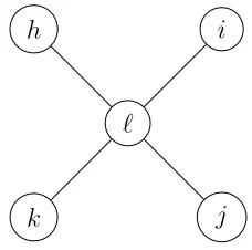
Example 1. There is a social network of 5 individuals arranged in a star as depicted
in Figure1. We label the peripheral players h, i, j, and k and the central player`.
h
k j
i
`
Figure 1: A 5-person star network
Each individual wishes to utilise the online media services provider Netflix. The
company’s rules permit any individual who purchases an account to stream
simultane-ously on a maximum of five devices. We assume that edges in the network represent
close friendships so that any person who purchases will and can share with each of his
friends. Formally, this is modelled as the simultaneous-move ‘best-shot game’ of
Gale-otti et al. (2010) where each agent has strategy set {0,1}, with 1 meaning purchase a
Netflix account and 0 meaning don’t.
It is a best-response for each agent to purchase a Netflix account if and only if
above. In the first, only the individual in the centre,`, purchases. In the second, all the
peripheral individuals, h, i, j, k purchase and the central individual ` does not. These
two equilibria are depicted in Figure2below, with adopters in blueand non adopters in
red. The direction of sharing is further indicated by arrows, with the tail of any arrow originating at a purchaser and the head of an arrow pointing to those with whom she
shares.
h
k j
i
`
h
k j
i
`
Figure 2: Equilibria for best-shot game on 5-person star network
Now let consider what would happen if Netflix altered the number of devices that one
account can simultaneously access. Let the number of people that may simultaneously
use the service other than the account holder be denoted by κ. An individual who
purchases an account can nominate only κ of her neighbours (and will nominate all of
her neighbours if she has less than κ). For κ = 1,2,3, the only equilibrium outcome
is for the peripheral individuals to purchase an account (and each to nominate the
central individual, `, as the friend who may use the account free of charge). These
equilibrium outcomes have a D-set of size 1 and are each depicted in the right hand
panel of Figure 2. The outcome depicted in the left hand panel is no longer supported by an equilibrium, the reason being that if ` purchases an account then she can only
nominate 3 of her 4 neighbours which will leave one without access. It is then optimal
for this un-nominated neighbour to purchase an account, but he in turn must nominate
` who subsequently would no longer want to purchase. So in this example, restricting
attention to equilibrium outcomes, the number of adopters in equilibrium can only
decrease as Netflix permit more “shareability”.
Example 2. The previous example suggests a natural conjecture. This is, loosely put,
that the size of D-sets will not increase as capacity increases. The following example
shows that this conjectures is not correct and also highlights some other interesting
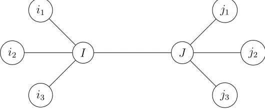
We imagine a couple Isabella and John, I and J, who are planning on introducing
their friends to one another at a gathering. We refer to Isabella’s friends as i1, i2, and
i3, and John’s friends as j1, j2, and j3. Isabella knows her friends and John knows
his friends; no other pair of individuals have previously met. This social network is
depicted in Figure 3.
i1
i2
i3
I J
j3
j2
j1
Figure 3: Two star graphs with central vertices connected
The gathering will take place at a restaurant outside of town and so people must
travel by car. While everybody owns a car and will drive if needs be, it is preferable to
get a ride than to drive oneself (one can then drink alcohol, save on fuel costs, save on
parking costs, etc.).
In this example, a person’s capacity is the number of passenger seats in their car.
For the sake of simplicity, let us assume that everybody’s car is the same size and
consider how the equilibria vary as capacities are increased. (Note that to economise
on space we are somewhat loose and describe equilibria by naming only the drivers,
i.e., the D-set.) When everyone’s car can give a ride to only one passenger, κ is equal
to 1 for everybody, there is only one equilibrium with D-set D1 = {i1, i2, i3, j1, j2, j3}.
For κ equal to 2, D1 is again the only D-set. When κ is increased to 3, three new
equilibria emerge. This collection of equilibria have D-sets given by D1, D2 = {I, J}
with Isabella offering a ride only to her three friends and John offering a ride to his
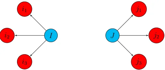
three friends,D3 ={i1, i2, i3, J} andD4 ={I, j1, j2, j3}. Thus forκ equal to 3, there is
an equilibrium with only two people driving. This equilibrium is depicted in Figure 4
below as a subgraph of the social network with drivers again inblue and passengers in
red, and arrows between the two originating at drivers offering a ride. Whenκincreases to 4, the model reduces to the best-shot game for which adopters in equilibrium form a
maximal independent set (the collection of which is D1, D3,and D4) for which at least
i1
i2
i3
I J
j3
j2
j1
Figure 4: Equilibrium with minimal number of adopters forκ= 3
We note some other interesting features illustrated by this example. First, when
κ is equal to 1 or 2, there is no equilibrium in which I or J drive which highlights
a difference between D-sets and maximal independent sets, since for any graph every
vertex is part of at least one maximal independent set. Second, and referencing the
original conjecture, the equilibrium with the fewest number of drivers occurs with κ
equal to 3 for each individual, at which point individuals I and J both have degree
greater than their capacity.7 Third, the number of equilibrium outcomes decreased as
κincreased from 3 to 4. Furthermore, while increasing capacity may lead to an increase
in the number of equilibria, it may remove the most efficient equilibrium (that with the
fewest drivers). Lastly, consider an amendment to the graph in Figure 3 such that i1 and i2 are friends. For κ = 1 there is an equilibrium with D-set D1 where 6 people
drive, but when capacity is maximal the largest D-set is the maximal independent set
of maximum size which has only 5 elements.
Example 3. The previous examples were special cases of the general model - those
where the action set is simply{0,1}(i.e., do not purchase / purchase, and do not drive
/ drive). In the general model, the action set is the set of non-negative integers and
there is a most-desired quantity that we denote byq∗. By “most desired” we mean that
once an individual’s total quantity received (his own action choice added to the action
choices of those who nominated him) reaches q∗, he is satiated.
In this richer model, there can be pure strategy equilibria where some individuals
choose a strictly positive action choice that is less thanq∗. We call equilibria in which
7Note that the size of the smallest D-set can not only change with capacity but can do so to an
individuals choose either action 0 or actionq∗ specialised. (In the first two examples q∗
was equal to 1, so all pure strategy equilibria were specialised.) We will show via an
example that pure strategy equilibria that are not specialised may not be stable.
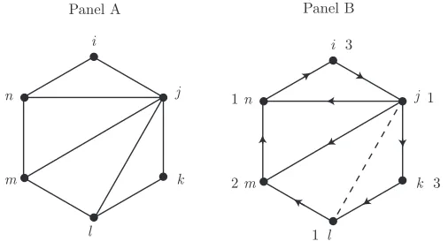
We consider a social network with 6 agents denoted i, j, k, `, m, and n. Individual
j is linked to everybody, individuals i and k are linked to j and one other, while all
other individuals are linked toj and exactly two others. This is depicted in Panel A of
Figure5 below.
i j k l m n i j k l m n 3 1 3 1 2 1 i j k l m n 0 4 0 0 0 4
Panel A Panel B Panel C
Figure 5: A 6 person network
In addition to the larger action space, this example is more complex in that we
allow capacities to differ across agents. Specifically, we suppose that the capacity forj
is equal to 3 and the capacity for all other individuals is equal to 1. Lastly, we suppose
that the optimal quantity of the good isq∗ = 4.
Panel B of Figure 5 presents a pure strategy that is not specialised, while Panel C presents a specialised equilibrium. Our focus is on the equilibrium in Panel B. All
agents choose positive quantities where the quantity is given by the number beside their
name. Arrows depict nominations with the number of arrows originating at each vertex
equal to that individual’s capacity. It is a pure strategy since, for every agent, the
sum of their quantity choice and the in-flow of quantities from other individuals who
nominate them is equal to 4 (=q∗).
Now we consider dynamics. We imagine that agentiunilaterally decreases his action
choice from 3 to 2. We label the time, t, at which this happens by 0. We label the
action profile at this time by x(0), where ordering the players as before we have that
x(0) = (x(0) i , x
(0) j , x
(0) k , x
(0) ` , x
(0)
the sequence of action profilesx(t)
t≥0 where for allt≥1, elements in the profilex (t)
is the best-action response for the relevant agent to x(t−1). Importantly, we imagine that the nominations of each agent are held fixed.
It is also important to emphasise that when it comes to studying dynamics, the
modeller must be aware of who each player nominates. The reason can be seen from
considering a specialised equilibrium. In the static case, it did not matter who those
that made an action choice of 0 nominated. But in the dynamic environment, if one
those individuals deviates in their action choice, then this will have repercussions that
can only be analysed if the nominations are known.
In turns of updating their action choice, the behavioural rule is one of myopic
best-response (in action, not nomination as this is held fixed). Specifically, each agent
examines the total currently being supplied to him. If this total is less than 4, then
he makes up the difference by increasing his own supply; if this total is more than 4
then he decreases his own supply. Thus in period 1, the only individuals who will alter
their action are i and j as each receive a total of 3 (i provides 2 himself and receives
1 from n who nominated him, while j provides 1 himself and receives 2 from agent i
who nominated him). Since both are 1 unit short of q∗ = 4, they will each increase
their period 0 action by 1. We thus get that x(1) = (x(1) i , x
(1) j , x
(1) k , x
(1) ` , x
(1)
m , x(1)n ) =
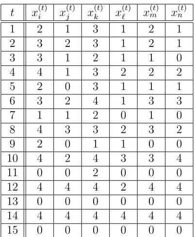
(3,2,3,1,2,1). The evolution of this behaviour can then be traced and is done in Table
3below.
We note that the action profiles evolve in a seemingly irregular way until period
13 at which point it starts to cycle between everybody choose 4 in even periods and
everybody choose 0 in odd periods. So population behaviour was initially at a
non-specialised equilibrium, one individual’s action choice was changed by 1 unit and then
all players were allowed to update. Surprisingly, this small deviation from the
non-specialised equilibrium led to a complete unravelling. In Proposition 2 we show that is not a coincidence. For every non-specialised equilibrium, if the action choice of any
t x(it) x(jt) xk(t) x(`t) xm(t) x(nt)
1 2 1 3 1 2 1
2 3 2 3 1 2 1
3 3 1 2 1 1 0
4 4 1 3 2 2 2
5 2 0 3 1 1 1
6 3 2 4 1 3 3
7 1 1 2 0 1 0
8 4 3 3 2 3 2
9 2 0 1 1 0 0
10 4 2 4 3 3 4
11 0 0 2 0 0 0
12 4 4 4 2 4 4
13 0 0 0 0 0 0
14 4 4 4 4 4 4
15 0 0 0 0 0 0
Table 1: Evolution of behaviour under best-action reply dynamic.
3
The Model
We begin with the graph theoretic terminology required to describe the model.
An undirected graph G = (V, E) consists of a nonempty finite set V = V(G) of
elements calledvertices and a finite setE =E(G) of unordered pairs of distinct vertices
called edges. We call V(G) the vertex set of G and E(G) the edge set of G. In other
words, an edge{i, j}is a 2-element subset ofV(G). We will often denote an edge{i, j}
byij. For edge ij ∈E(G) we say that i and j are the vertices, and say that
end-vertices are adjacent. We say that vertex i is incident to edge e if it is an end-vertex
of e. A graph G on n vertices is called complete if every two distinct vertices in G are
adjacent; Gwill be denoted by Kn.
A path in a G is a finite sequence of edges which connect a sequence of distinct
vertices. A graph is connected if there is at least one path containing each pair of
vertices. We define the neighbourhood of a vertex i, NG(i), in a graph G to be the set
of vertices that vertex i is adjacent to, NG(i) = {j ∈V : ij ∈E}, and we say that
vertexj ∈NG(i) is aneighbour of vertex i; we writedG(i) for the cardinality ofNG(i).
For a connected graph with at least two vertices, the neighbourhood of every vertex is
With the above we can now introduce the game theoretic model. In the model,
vertices are interpreted as players and edges represent connections between pairs of
players. We assume the population (vertex set) is of size n and that the graph G is
connected.
LetX ={0,1, . . . ,x¯}denote the finite set of actions common to each agent. Actions
have both a private and (local) public benefit, but only a private cost. WritingN0 for
the set of non-negative integers, there is a capacity function κ:V →N0 that specifies,
for each player, how many of his neighbours may benefit from his action choice. This
subset of neighbours are said to be nominated. If a player’s capacity is zero then he
nominates no neighbours; if a player’s capacity is at least as great as his degree then all
of his neighbours are nominated. Formally, for any nonempty set A and nonnegative
integerk, we denote by [A]k the collection of k-subsets of A. That is, [A]k={A}when
k≥ |A|, [A]k={S ⊆A : |S|=k} when 0< k < |A|, and [A]k =∅ when k = 0. With
this, player i’s set of pure strategies is given by Xi ×M (κ)
i , with M (κ)
i = [NG(i)]κ(i)
representing the collection of subsets of NG(i) of size κ(i).
We writexi for individuali’s action choice fromX, andmi for his nominating choice
fromMi. (Note we omit the superscript (κ) of Mi(κ) whenever no confusion arises.) A pure strategy profile is represented by a vector (x,m) = (x1, . . . , xn),(m1, . . . , mn)
specifying an action and a set of nominees for each agent. (We callx the action profile
and mthe nomination profile.)
Given the above, the utility to player i,Ui, from strategy profile (x,m) is given by
Ui x,m
=fxi+
X
{j∈NG(i) :i∈mj}
xj
−cxi (1)
where we assume that (i)c >0, and (ii) there exists a q∗ ∈X such that
q∗ ∈argmax
x∈X
(f(x)−cx) and f(x)−cxis non-increasing for x≥q∗.
Note that this definition implies that it makes no sense for a player i to increase
xi if xi + P{j∈NG(i) :i∈mj} = y ≥ q
∗ as f(y+ t) −c(y+ t) ≤ f(y)− cy and thus
f(y+t)−ct≤f(y). Thus, each player i chooses an actionxi ∈Xi and decides which
neighbours to share with via the choice mi ∈ Mi. Note that player i’s utility solely
nominate him. Playeri’s utility does not depend upon who he himself nominates.
The utility function as defined in (1) is very general. It does not require concavity of f as in that of Bramoull´e and Kranton (2007). If we take X = {0,1}, f(x) = 1
for all x ≥ 1, and 0 < c < 1, then the game becomes the “Netflix Game with κ-user
sharing rule”.
A pure strategy Nash equilibrium is defined in the usual way.
Definition 1. A strategy profile (x∗,m∗) is a pure strategy Nash equilibrium if for
every i= 1, . . . , n, and every xi ∈Xi and everymi ∈Mi we have
Ui((x∗,m∗))≥Ui (x∗1, . . . , x
∗
i−1, xi, x∗i+1, . . . , x
∗
n)(m
∗
1, . . . , m
∗
i−1, mi, m∗i+1, . . . , m
∗
n)
.
We have the following:
Proposition 1. A pure strategy Nash equilibrium exists for any graph G and any
capacity function κ:V →N0.
While the above is a strong result, we will focus on what, followingBramoull´e and
Kranton(2007), we term specialised strategy profiles - those in which each agent either
choose actionxi = 0 or xi =q∗. We have the following definition.
Definition 2. A specialised strategy profile is a pure strategy profile in which for all
i∈V we have either xi = 0 orxi =q∗.
We emphasise that specialised strategy profiles do not say anything about
equilib-rium since for that we must also know who nominated who. For example, all individuals
choose action 0 is specialised but clearly not an equilibrium. We begin building up to
such a definition now.
For a given specialised strategy profile (x,m), let D(x,m) = {i∈V :xi =q∗} be
those agents who supply q∗, and P(x,m) = {i∈V :xi = 0}, where we interpret D
and P as Drivers and Passengers respectively (Drivers provide while Passengers free
ride). Clearly, at any specialised strategy profile, we have that both D∩P = ∅ and
D∪P = V. However, we aim to go further. In words, we wish to find a strategy
profile such that nobody inD is nominated by somebody else inD, and everyone in P
is nominated by at least on person inD.
Some additional graph theoretic terminology is required. Given a graph G =
and E(H) ⊆ E(G). If V(H) = V(G) we say that H is a spanning subgraph of G. A
subgraph H is said to be induced by a subset S of vertices of G= (V, E), if the vertex
set of H is S and the edge set consists of all edges in E that have both end-vertices
in S. If G = (V, E) is a graph and S ⊆ V(G), then G−S is the subgraph induced
by V(G)\S. For a subgraph H of G, we define G−H as G−V(H). Similarly, for
edges, ifB ⊆E(G), thenG−B is the spanning subgraph ofGwith edge setE(G)−B.
A bipartite graph is a graph whose vertices can be partitioned into two disjoint sets
(called partite sets) A and B such that every edge has one end-vertex in A and the
other inB. A bipartite graph G with partite sets A and B is calledcomplete bipartite
if ab ∈ E(G) for every a ∈ A and b ∈ B. Then G is denoted by K|A|,|B|, where |A|
and |B| are the cardinalities of setsA and B. A complete bipartite graph K1,p (p≥2)
is called a star, the vertex adjacent to all other vertices the center, all other vertices
leaves. For example the graph in Figure 1 is a star with center `.
Abstracting from the actions chosen by the individuals, we wish find a spanning
bipartite subgraph,H, of G, with partite sets D and P such that there does not exist
an i ∈ D such that i ∈ mj for any j ∈ D, and for all i ∈ P there exists at least one
j ∈D such thati∈mj. This leads us to the following definition.
Definition 3. A spanning bipartite subgraph H of G with partite sets P and D is
called aκ-DP-subgraph(or, simply aDP-subgraphif the functionκis fixed) if for each
i∈D the degree ofi inH is min{κ(i), dG(i)}and for every i∈P the degree of iin H
is positive.
With this, we can define what it means for a strategy profile to be a balanced
specialised profile as follows.
Definition 4. A specialised profile (x,m) is a balanced specialised profile supported
byκ-DP-subgraph H of Gif
xi =q∗, mi =NH(i) if i∈D
xi = 0, mi =S for someS ∈M (κ)
i if i∈P
When it comes to adding dynamics, we will not only examine balanced specialised
profiles, but we will also require that every vertex in P nominates at least one of the
Definition 5. A specialised profile (x,m) is a nicely balanced specialised profile
sup-ported byκ-DP-subgraph H of Gif
xi =q∗, mi =NH(i) if i∈D
xi = 0, mi =S for some S∈M (κ)
i such that S∩NH(i)6=∅ if i∈P
We now have the following theorem, which is an improvement of Proposition 1.
Theorem 1. For any graph G and common utility function as given by (1), there exists a nicely balanced specialised profile and all nicely balanced strategy profiles are
pure strategy Nash equilibria.
Proof. The proof has two parts. The first is to show that every graph G possesses at
least one κ-DP-subgraph. The second is then to show that a nicely balanced strategy
profile induced byκ-DP-subgraph involves each agent choosing the optimal action.
Here we prove the following statement: If G is a graph and κ : V(G) → N0 is a
function, thenG has a DP-subgraph.
The proof proceeds by induction on the number n of vertices ofG.Ifn= 1, then G
is a DP subgraph withD=V(G) and P =∅.
Now assume the claim is true for all graphs with fewer thann0 ≥2 vertices, and let
Gbe a graph on n0 vertices.
Case 1: There is a vertex i of degree at most κ(i). LetB be the star with
cen-teriand leavesNG(i),whereNG(i) is the neighbourhood ofiinG. LetG0 =G−B.
SetD={i}andP =NG(i).IfG0has no vertices thenBis clearly aDP-subgraph
of G.
Otherwise, by induction hypothesis, G0 has a DP-subgraph H0 with partite sets
P0 and D0. Construct a subgraphH of Gfrom the disjoint union of H0 andB by
adding to it for everyj ∈D0 withdG0(j)< κ(v),exactly min{dG(j), κ(j)}−dG0(j)
edges of G between j and N(i).Set D=D0 ∪ {i}and P =P0∪N(i).
To see that H is aDP-subgraph of G,observe that (a)H is a spanning bipartite
subgraph ofG asH0 andB are bipartite and the added edges are betweenDand
P only, (b) every vertex j ∈ D has degree in H equal to min{κ(j), dG(j)}, (c)
Case 2: For every vertex j ∈V(G), dG(j)> κ(j). Let i be an arbitrary vertex.
Delete dG(i) − κ(i) edges incident to i and denote the resulting graph by L.
Observe that every DP-subgraph of L is a DP-subgraph of G since no vertex in
L has degree less than κ(i). This reduces Case 2 to Case 1.
To complete the proof it remains to show that a nicely balanced strategy profile
induced by aκ-DP-subgraph is a Nash equilibrium. Let (x∗,m∗) be a nicely balanced
specialised profile. As mentioned before, we note that the utility function defined in
(1) does not depend on mi. Thus player i cannot increase her payoff by deviating
from m∗i. If i ∈ D then by the definition of a nicely specialised profile induced by a
κ-DP subgraph, we have x∗i = q∗ and P
{j∈NG(i):i∈m∗j}x
∗
j = 0. Thus is follows from
the definition of the utility of i that for all x that are obtained from x∗ by replacing
x∗i =q∗ by any t >0, we have
Ui(x∗,m∗) = f(q∗)−cq∗ ≥f(t)−ct=Ui(x,m∗).
If i ∈ P then x∗i = 0 and P
{j∈NG(i):i∈m∗j}x
∗
j = sq
∗ for some s > 1. Thus by the
observation just after the definition of the utility function, for all x that are obtained
fromx∗ by replacingx∗i = 0 by any t >0 we calculate
Ui(x∗,m∗) =f(sq∗)≥f(sq∗+t)−ct=Ui(x,m∗).
We now make some observations about Theorem1and in particularκ-DP-subgraphs and their associatedD-sets and P-sets.
Fix a graph G= (V, E). An independent set is a subset of vertices no pair of which
are adjacent, and amaximal independent set is an independent set that is not a proper
subset of any other. Adominating set is a set of vertices such that every vertex in V
is either in the set or has a neighbour in the set, and a minimal dominating set is a
dominating set that does not contain a proper subset that is dominating. (Note that
the notion of dominating is defined only for sets whereas our concept of nominating
is defined for individual vertices and by considering multiple nominating vertices can
dominating sets. For a further discussion of some of the properties of D-sets, refer to
AppendixA.
Clearly a D-set is a dominating set though the reverse need not hold. Indeed, in
a complete graph Kn every vertex forms a dominating set, but if κ(i)< d(i) for every
i∈V(Kn), then no singleton can be a D-set. We will add further observations. First,
as with dominating sets but not independent sets, it is possible that two vertices inD
are adjacent in G. An instance of this was seen in the second example of Section 2for the equilibrium in which the only adopters two central vertices were the only adopters.
Second, when κ(i) ≥ dG(i) for all i, we have that D is a maximal independent set
(which is by definition dominating). Third, and related to the previous observation,
is that unlike maximal independent sets, for a given graphG and capacity function κ,
oneD-set may be a strict subset of another. As an example consider a complete graph
with 5 vertices i, j, k, l, and m with κ = 2 for each vertex. One such D-set is {i, j, k}
with each nominatingl and m, while anotherD-set is {i, j} withi nominatingk and l
and j nominating l and m. Finally we note that the procedure described in the proof
of Theorem1allows us to find a D-set in polynomial time. Note, however, that such a procedure may not find all D-sets of a given graph G. For example the D-set given in
Example2 consisting of I and J would never be found.
4
Efficiency and Comparative Statics
In this section we focus on the efficiency of balanced specialised profiles. For a given
graph and a given capacity functionκ, there are often multiple balanced strategy
pro-files, so our attention is on those with the smallest and largestD-sets (that we interpret
this a measure of efficiency/inefficiency). We then consider how incremental
amend-ments to the model will affect such (in)efficiency. There are two natural ways to amend
the model. The first is to incrementally increase the capacities of the agents, while the
second is to alter the underlying graph, G, either by adding/deleting an edge or by
adding/deleting a vertex and all the edges it is incident to.
Recall that for a specialised strategy profile (x∗,m∗), D(x,m) denotes the set of
individuals who adopt. We say that a balanced specialised profile (x,m) is efficient if
its associated D-set is of minimal size, and inefficient if it is of maximal size.8, Clearly
not every nicely balanced strategy profile is efficient. For a graph G and capacity
functionκ:V →N0, letδminκ (G) andδmaxκ (G) denote the minimum and maximum sizes of D-sets of G.
First, we will show that computingδminκ (G) andδmaxκ (G) are unfortunately NP-hard problems. Indeed, ifκ(i)≥d(i) for every vertex iin a graphG, then δminκ (G) (δκmax(G), respectively) equals the minimum (maximum, respectively ) size of an independent set
of vertices inG, whose computation is NP-hard (see, e.g., Garey and Johnson (1979))
for both minimum and maximum.
We wish to see how the sizes of such sets co-evolve as the player’s capacities are
increased.To this end, let κ0 : V(G) → N0 be a function such that κ(i) ≤ κ0(i) for
everyi∈V(G). We compareδminκ (G) andδmaxκ (G) with δκmin0 (G) andδmaxκ0 (G).Theorem
2 shows a particular inequality holds for every graph G. Unfortunately, none of the other three possible inequalities can hold as we have seen with some examples.9
Theorem 2. For every graph G, δκ0
min(G)≤δκmax(G).
Proof. Let κ+ : V(G) →
N0 be function such that κ+(i) =κ(i) for i ∈ V(G)−j and
κ+(j) = κ(j) + 1 for some j ∈ V(G). To prove the theorem is sufficient to show that
δminκ+ (G)≤δmaxκ (G).
We proceed by induction on n+m, where n is the number of vertices of G and
m is the number of edges in G. If n+m = 1, then G consists of a single vertex and
settingD=V(G) and P =∅gives the only DP-subgraph for both κand κ+. We may
assume that G is connected as otherwise we can consider its components and apply
the induction hypothesis on the component containing j and the vertices in the other
components have the same values forκ and κ+. Let G=K1,n−1, wheren ≥2 and j is the center of the star. If κ+(j)≥n−1, then δκmin+ (G) = 1 and we are done. Otherwise,
V(G)−j is a D-set for bothκ and κ+.
is weakly efficient if there does not exist another balanced specialised profile (x∗∗,m∗∗) such that
D(x∗∗,m∗∗)⊂D(x∗,m∗). Note further that such a definition is not useful with the best-shot game since by definition any two maximal independent sets do not have the set inclusion property.
9The graph in Example2showed that the smallestD-set can both decrease and increase as capacity
increases. We also saw that the largestD-set can decrease in the same example by adding an edge between any pair of Isabella’s friends. To see that the largestD-sets can increase in size consider the complete graphK7 on 7 vertices. Pick two 2 verticesi, j and letκ(i) =κ(j) = 2 andκ(x) = 6 for all other verticesx. Then all equilibria haveD-sets of size 1 (and all vertices excepti andj can form a
D-set) and thus δκmax(G) = 1. But if we increaseκ(i) by one to obtain a new capacity function κ+
theni, jform aD-set andδκ+
Now we may assume that n≥3, Gis connected and there is an edge in G which is
not incident toj. Consider two cases.
Case 1: There is a vertex i∈V(G)−j of degree at most κ(i). LetBbe the the
star with center i and leavesNG(i),where NG(i) is the neighbourhood ofi in G.
Let G0 = G−B. Set D = {i} and P = N(i). If G0 has no vertices then B is
clearly a κ-DP-subgraph and κ+-DP-subgraph of G.
Otherwise, by induction hypothesis,δk+
min(G
0)≤δk max(G
0), wherekisκrestricted to
G0. The two correspondingDP-subgraphs of G0 can be extended to those ofGby
adding ito their D-sets andN(i) to their P-sets and adding to every` ∈Dwith
dG0(`)< κ(`), and dG0(`)< κ+(`), respectively, exactly min{dG(`), κ(`)} −dG0(`)
or exactly min{dG(`), κ+(`)} −dG0(`) edges of Gbetween ` and N(i). Thus,
δminκ+ (G)≤δmink+ (G0) + 1≤δmaxk (G) + 1≤δmaxκ (G).
Case 2: The degree of every vertex i∈V(G)−j is larger than κ(i). Choose any
edge i` such that j 6∈ {i, `} and delete it from G. By induction hypothesis, for
the resulting graph G0 we have δmink+ (G0) ≤ δmaxk (G0). It remains to observe that the two DP-subgraphs of G0 are also DP-subgraphs of G (the functions κ and
κ+ were not changed and the deleted edges are not needed).
5
Stability of Specialised Profiles
In this section we introduce dynamics with the goal of examining which strategy profiles
are robust to unilateral deviations. Recalling that an agent’s utility is unaffected by his
choice of nomination, the number of best-responses for each agent may be enormous. As
such, throughout we will assume the nominating profile is fixed and consider only the
what action choices are optimal given the nominating profile and the action choices of
others. We call this restricted best-response abest-action response. Given a nomination
profile m and the action profile x, it is not hard to see that the best-action response
of agent i, Bi,m(x), is given by
Bi,m(x) = max
q∗− X
{j∈Ni(G) :i∈mj}
xj, 0
We extend this to the best-action reply dynamicBm :X →X as
Bm(x) =
B1,m(x),B2,m(x), . . . ,Bn,m(x)
Definition 6. Given an action profile xwe define thebest action evolution of x
recur-sively byx(0) =xand for t ≥1,x(t) =B
m(xt−1).
We are interested in comparing population level contributions. As such we will wish
to order action profiles wherever possible. For any two action profiles x,x0 ∈ X, we
say x ≥x0 if xi ≥ x0i for all i∈ {1, . . . , n}, and x> x0 if xi ≥yi for all i∈ {1, . . . , n}
and xj > yj for at least onej ∈ {1, . . . , n}.
We then have the following results.
Lemma 1. Suppose that (x∗,m∗) is a pure strategy Nash equilibrium and let x≤x∗.
Then the best action evolution of x satisfies for all t ≥0
(i) x(t+1) ≥x∗ ≥x(t) if t is even.
(ii) x(t+1)≤x∗ ≤x(t) if t is odd.
Proof. Let t = 0. Then by assumption x(0) ≤ x∗. If we choose i to be an individual
with x∗i = 0, then clearly we have x(1)i ≥ 0 =x∗i = 0. Now, let i be an individual with
x∗i 6= 0. Then
x∗i =q∗− X
{j∈NG(i):i∈mj}
x∗j ≤q∗− X
{j∈NG(i):i∈mj}
x(0)j =x(1)i .
Thusx(1)i ≥x∗i and x(1) ≥x∗. By considering individuals with x(2) 6= 0 separately, we can use the same argument to shows that x(2) ≤ x∗. Thus we have x(2) ≤ x∗ ≤ x(1).
The result then follows easily by induction.
Lemma1implies that if we take a pure strategy Nash equilibrium action profile x∗, for anyx≤x∗ the best action evolution ofxeither oscillate aroundx∗ forever, or there
exists ant0 such that for all t≥t0, x(t) =x∗. Note that this is the case as we consider only finite networks and so there are only a finite number of different possibilities for
the xt and therefore they have to repeat. This motivates the following definition.
Definition 7. We say that the best action evolution of x settles in x∗ if there exists
We emphasise that Lemma 1 holds for all Nash equilibrium strategy profiles and not simply specialised ones. While Lemma 1 is a statement about the population action profiles, the next two results, Lemmas2and 3are statements about best-action responses at the level of the individual. We emphasise again that both results apply
to all pure strategy Nash equilibria, not simply specialised ones. The first lemma is an
immediate corollary of Lemma 1.
Lemma 2. Suppose that (x∗,m∗) is a pure strategy Nash equilibrium. Let x < x∗.
Then the best action evolution of x satisfies the following:
(i) If t is odd, then xi(t)6= 0, for all i such that x∗i >0, and
(ii) If t is even, then x(it) 6=q∗, for all i such that xi < q∗.
We will need the following lemma which essentially says that a state` reacts to any
changes of states that affect it unless ` does not need to provide anything, that is x`
can remain zero and is still satisfied.
Lemma 3. Suppose that (x∗,m∗) is a pure strategy Nash equilibrium. Let x≤ x∗ be
an action profile and consider the best action evolution of x. Let ` be nominated by i,
that is ` ∈mi.
If x(`t)>0 and x(it) > xi(t−1), then x(`t+1) < x(`t) (3)
If x(`t+1) >0 and x(it) < xi(t−1), then x(`t+1) > x(`t) (4)
Proof. We first show (3). So assume x(it) > xi(t−1). Then, by Lemma 1, t must be odd. Now, again using Lemma 1, we have for ` ∈mi
X
{j∈NG(`):`∈mj}
x(jt)− X
{j∈NG(`):`∈mj}
x(jt−1)
=x(it)−x(it−1)+ X
{j∈NG(`) :`∈mj, j6=i}
x(jt)− X
{j∈NG(`) :`∈mj, j6=i}
x(jt−1)
≥x(it)−x(it−1)
Rearranging and addingq∗ to both sides of this inequality gives that
q∗− X
{j∈NG(`):`∈mj}
x(jt) < q∗− X
{j∈NG(`):`∈mj}
x(jt−1).
But note that by the best-action response (2) and because we assume thatx(`t) >0 the right hand side is equal tox(`t). Alsox(`t+1) equals either the left hand side of the above inequality or is equal to zero and in both cases is smaller than x(`t). The inequality in (4) is shown in a similar manner.
We now introduce our notion of stability when the nominating profile is held fixed
and actions are updated according to the best-action reply dynamic. In words, we say
that action profile xis stable relative to the nomination profile m, if, when the action
of any individual is changed by some strictly positive amount, repeated application of
the best-action reply dynamic will lead population behaviour back to action profilex.
Definition 8. We say that strategy profile (x,m) is action stable if there existsδ ≥1
such that for any i = 1, . . . , n and any action profile x0 with xj = x0j for j 6= i and
|x0i−xi| ≤δ the best action evolution ofx0 settles in x.
In other words a strategy profile is action stable if one can change any one coordinate
by at mostδ and the best action evolution will settle inx. The following result shows
that any pure strategy Nash equilibrium profile that is not balanced specialised is not
action stable and thus, a strategy profile being balanced and specialised, supported by
aκ-DP-subgraph, is necessary for action stability.
Proposition 2. Suppose that (x∗,m∗) is a pure strategy Nash equilibrium such that
0< x∗` < q∗ for some `. Then (x∗,m∗) is not action stable.
Proof. DefineL:=j : 0< xj∗ < q∗ . By assumption` ∈L. First we will show that `
cannot be the only element in the set L. This is immediate since
0< x∗` =q∗− X {j∈NG(`) :`∈m∗j}
x∗j < q∗ =⇒ 0< X
{j∈NG(`) :`∈m∗j}
x∗j < q∗.
Thus, there exists some j ∈ L such that j ∈NG(`), ` ∈m∗j. It follows that there exist
indices i1, i2, . . . , ik such that i1 ∈m∗i2, i2 ∈ m
∗
i3, . . . , ik−1 ∈ m
∗
ik and ik ∈m
∗
readers familiar with graph theory we can build a directed graph onLwith an arc from
j toiifi∈m∗j. The above result implies that every vertex has at least one in-neighbour and hence the graph contains a cycle.) By renaming if necessary we may assume that
ij =j for allj = 1, . . . , k, so fori = 1, . . . , k we have i∈ L, i∈m∗i+1 and k ∈m∗1. We definex by subtracting 1 from the first coordinate of x∗, that is,
x= (x∗1 −1, x∗2. . . , x∗n).
We claim that x does not settle in x∗. We prove the claim by contradiction. In
particular we assume that there exists a (minimal)t0 such that for allt ≥t0 and for all
i= 1, . . . , k, we havex(it) =x(it+1). Note that t0 ≥ 1 as x (0) 1 =x
∗
1−16=x
∗
1 =x (1) 1 . Also for all i = 1, . . . , k, we have x(t0)
i = x (t0+1)
i = x
∗
i > 0. The contradiction now follows
from Lemma3 by choosingi∈ {1, . . . , k}such that xt0−1
i 6=x t0
i and ` =i+ 1. Such an
iexists as we have chosen t0 minimal.
While Proposition 2 says that balanced specialised profiles are necessary for sta-bility, the following result, Proposition 3 shows that they are not sufficient. However, Proposition4shows that balanced specialised profiles supported by a κ-DP-subgraphs with a mild density condition are sufficient for stability.
Proposition 3. Suppose (x∗,m∗) is a nicely balanced specialised profile induced by
κ-DP-subgraph H of G, and suppose further that dH(i) = 1 for some i ∈ P. Then
(x∗,m∗) is not stable.
Proof. Without loss of generality we may assume that 1∈P, dH(1) = 1 and that 2 is
the neighbour of 1 in H. Note that x∗2 = q∗ as the strategy profile is nicely balanced
and specialised. Consider
x= (x∗1, x∗2−1, . . . , x∗n) = (x∗1, q∗−1, . . . , x∗n).
We claim that x does not settle in x∗. To see this we prove by induction that for
all odd t we have x(1t) > 0 and for all even t we have xt 2 < q
∗, Clearly this is true for
t= 0 and also for t= 1 as the best action response for 1 is x(1)1 = 1>0. Now assume
that the statement is true for allt ≤t0 with t0 ≥2.
If t0 is even then by induction hypothesis xt20 < q∗ and by Lemma 1 for all j ∈ P we have x(t0)
j ≤x
∗
j = 0 and thus x (t0)
elements in P, the best action response for 1 is x(t0+1)
1 =q
∗−x(t0)
2 >0.
Ift0 is odd then by induction hypothesisxt10 >0 and by Lemma 1 for all j ∈Dwe have x(t0)
j ≥ x∗j = q∗ and thus x (t0)
2 = q∗. Since 2 is nominated by 1 the best action response for 2 is x(t0+1)
2 ≤q∗−x (t0)
1 < q∗.
Thus, if there exists a nicely balanced specialised profile with an individual in P
who is nominated by only one agent inD, then the equilibrium is not stable. However,
the following proposition shows that if all individuals in P are nominated by at least 2
individuals inD, then the equilibrium is action-stable.
Proposition 4. Let q∗ ≥ 2. Suppose (x∗,m∗) is a nicely balanced specialised profile
induced by κ-DP-subgraph H of G, and suppose further that dH(i) = 2 for all i ∈ P.
Then (x∗,m∗) is stable.
Proof. Choose ε= 1. We must consider deviations by those in D and those in P. We
begin with those inD.
Case 1: i∈D. By definition x∗i =q∗. There are two subcases: Either we increase x∗j
by one or we decrease x∗j by one. In the first case, i.e. xsatisfiesx(0)i =x∗i + 1 =
q∗+ 1 and for all j 6=i, x(0)j =x∗j, it is immediate that Bm∗(x) =x∗.
In the second case let x satisfyx(0)i =x∗i −1 =q∗−1 and for all j 6=i, x(0)j =x∗j. By our assumption for all j ∈ P there is at least one neighbour k 6= i, k ∈ D
with j ∈ m∗k and thus maxnq∗−P
{k∈Nj(G) :j∈mk}xk, 0 o
= 0. It follows that
x(1)j = 0 for all j ∈ P. For all j ∈ D we have x(1)j =q∗ by Lemma 1 (or one can just observe only vertices in k∈P are nominatingj and all these vertices satisfy
x(0)k = 0).
Case 2: i∈P. By definition x∗i = 0, so the only deviation is to choose x(0)i = 1 and for all j 6=i,x(0)j =x∗j. Then
B`,m∗(x(0)) =
0, 0 if `∈P,
q∗−1>0, ` ∈NH(i)∩D,
q∗, ` ∈D\NH(i)
in the nominating network will behave in period 1. We have
X
{j∈NG(h) :h∈mj}
x(1)j = X
{j∈NG(h) :h∈mj}
Bj,m∗(x(0))
≥dH(h)(q∗−1)
≥2(q∗−1)
≥q∗
where the last inequality follows since q∗ ≥2. And thus, Bh,m∗(x(0)) = 0.
Furthermore, SinceH is aκ-DP-subgraph, we have thatNH(i)⊆P for all i∈D,
and thus the set {j ∈NG(i) : i∈mj} ⊆P for alliin D. Thus, for all`∈D, we
must have that B2
`,m∗(x(0)) = q∗ since Bi,m∗(x(0)) = 0 for all i∈P.
Therefore, (x∗,m∗) is stable.
6
Conclusion
This paper introduces a network model of public goods in which individuals face a
capacity constraint as to how many neighbours they may share with. Each agent
much decide how much of the good to provide and which subset of his neighbours to
share with. We focus on a subclass of pure strategy equilibria, that we term specialised
equilibria, wherein each agent provides either the most desirable quantity (is a ‘Driver’)
or provides nothing (is a ‘Passenger’). Interestingly, as capacities are increased the
number of Drivers across specialised equilibria need not decrease.
The model has a second interpretation wherein the nomination component is viewed
as pure network formation, with public good provision then occurring via the realised
network. Our model is thus one of the first to have a network formation component
coupled with a rich underlying game. While we introduce dynamics later in the paper,
we do so with the nomination component held fixed. Relaxing this would yield the
first model (to our knowledge) that captures the coevolution of behaviour and network
APPENDIX
A
Properties of
D
-sets
First we show some upper and lower bounds on the sizes ofD-sets for all graphs. Subsequently we look at specific classes of graphs that are commonly studied. The following definitions are required. For a
G= (V, E) be a graph and capacity functionκ:V →N0, we defineκ= miniκ(i), ¯κ= maxiκ(i), and
dG := minidG(i). Furthermore, lettingRdenote the real line, we define the ceiling and floor functions
as follows: for anyx∈R, letdxe:= min{n∈N|x≤n}and letbxc:= max{n∈N|x≥n}.
A.1
Bounds on
D
-sets
Lemma 4. Let G= (V, E)be a graph and κ:V →N0 be a capacity function. Then for any κ-DP -subgraphH of Gwe have,
(i) |D∪P| ≤(1 + ¯κ)|D|
(ii) |D∪P| ≥ |D|+ min{κ, dG} Proof. (i) We have
|V|=|D∪P|
=|D|+|P| ≤ |D|+X
i∈D
min{κ(i), dG(i)}
≤ |D|+X i∈D
κ(i)
≤ |D|+ ¯κ|D|
= (1 + ¯κ)|D|
(ii) For anyi∈D we have thatNH(i)⊆P. As such
|V|=|D∪P| ≥ |D|+NH(i)
=|D|+ min{κ(i), NG(i)} ≥ |D|+ min{κ, dG}
Recall that for a given graphGand given capacity functionκ,δκmin(G) andδκmax(G) represent the size of minimum and maximum D-sets taken over all κ-DP-subgraphs of G. We have the following lemma.
Lemma 5. Let G= (V, E)be a graph andκ:V →N0 be a capacity function. Then we have (i)δκ
min(G)≥ |V| 1+¯κ.
(ii)δκmax(G)≤ |V| −min{κ, dG}.
Proof. (i) Suppose to a contradiction thatδκ
min(G)< |G|
(ii) Suppose, again to a contradiction, that δk
max(G)>|V| −min{κ, dG}. Then there exists aκ-DP -subgraphH ofGwithD-setDsuch that|D|>|V| −min{κ, dG}=|D∪P| −min{κ, dG}which is a contradiction to part (ii) of Lemma 4.
Remark 1. For Lemma5, we need
|G| −min{κ, dG} ≥
|G|
1 + ¯κ ⇐⇒ (1 + ¯κ)(|G| −min{κ, dG})≥ |G|
To show this, first observe that
¯
κ+ ¯κ(|V| −1)≥min{κ, dV}+ ¯κmin{κ, dG} (5)
because ¯κ≥κand|V| −1≥dG(i) for alli. By rearranging (5), we find that This follows because
¯
κ|V| −(1 + ¯κ) min{κ, dG} ≥0 ⇐⇒ (1 + ¯κ)(|V| −min{κ, dG})≥ |V|
Now, putting Lemmas4 and5together, we obtain the following proposition.
Proposition 5. Suppose that κ(i)≤dG for somei. Then we have
l |V|
1 + ¯κ
m
≤δminκ (G)≤δκmax(G)≤ |V| −κ
Proof. The middle inequality is true by definition, while the left and right inequalities come from Lemma5parts (i) and (ii) respectively.
Proposition5holds for all graphs. However, we can improve upon those bounds for various classes of graph. This is the purpose of the following subsection.
A.2
D
-Sets for complete graphs
In this subsection we suppose thatG= (V, E) is a complete graph and that all individuals have the same capacity so that 1≤κ(i) =k≤ |V| −1 for alli∈V.
Given this we have dG =|V| −1 and thus mini{κ(i), dG} = min{κ, dG}=k for alli∈V. Thus from Proposition5 we obtain the following bounds,
l |V|
1 +k
m
≤δminκ (G)≤δκmax(G)≤ |V| −k (6)
In particular, ifk=|V| −1, then
δminκ (G) =δκmax(G) = 1
To achieve the lower bound, choosel1+|V|kmindividuals fromGand designate these individuals as
D. Now define letR=V\D. Then, using that
|V| −k≥l |V|
1 +k
m
⇐⇒ |V| −l |V|
1 +k
m
≥k,
andl1+|Vk|m≥1 (sincek≤ |V| −1) and
|V|
1 +k ≤
l |V|
1 +k
m
⇐⇒ |V| −l |G|
1 +k
m
≤l |G|
1 +k
m
k
we obtain
k≤ |R| ≤l |V|
1 +k
m
k.
That is, there are leastk agents inR and at mostd1+|Vk|ek. Thus, since Gis a complete network, we make each agent inD nominatekagents inR such thatD∪R=Gand obtainκ-DP-subgraph ofG. For the upper bound, we choose |V| −k individuals as elements inD. Then there exists exactly
kremaining individuals that we refer to asP. SinceGis a complete graph, we make it such that all individuals inDnominate each of thekremaining agents inP and obtainκ-DP-subgraph ofG. Thus we obtain the following proposition.
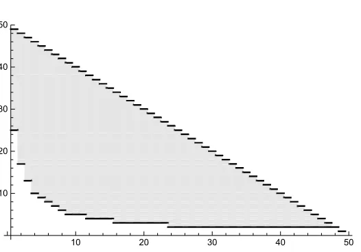
Proposition 6. Suppose that G= (V, E) is a complete graph and 1 ≤κ(i) =k ≤ |G| −1 for all i. Then we have
l |V|
1 +k
m
≤δminκ (G)≤δ κ
max(G)≤ |G| −k. (7) Moreover there exist bipartitek-DP-subgraphsH andH¯ with partite sets(D, P)and( ¯D,P¯)such that
|D|=l |V| 1 +k
m
and|D¯|=|V| −k
10 20 30 40 50
10 20 30 40 50
References
Yann Bramoull´e and Rachel Kranton. Public goods in networks. Journal of Economic Theory, 135 (1):478–494, 2007. URLhttp://www.sciencedirect.com/science/article/B6WJ3-4M0J4YN-1/ 2/2fd0550762d85d43f3b10d0a59e5116e.
Timothy G. Conley and Christopher R. Udry. Learning about a new technology: Pineapple in ghana. American Economic Review, 100(1):35–69, September 2010. doi: 10.1257/aer.100.1.35. URLhttp: //www.aeaweb.org/articles.php?doi=10.1257/aer.100.1.35.
P. Erd˝os and A. R´enyi. On random graphs i. Publicationes Mathematicae Debrecen, 6:290, 1959.
Andrew D. Foster and Mark R. Rosenzweig. Learning by doing and learning from others: Human capital and technical change in agriculture. The Journal of Political Economy, 103(6):1176–1209, 1995. ISSN 00223808. URLhttp://www.jstor.org/stable/2138708.
Andrea Galeotti, Sanjeev Goyal, Matthew O. Jackson, Fernando Vega-Redondo, and Leeat Yariv. Network games. The Review of Economic Studies, 77(1):218–244, 2010. doi: 10.1111/j.1467-937X. 2009.00570.x. URLhttp://restud.oxfordjournals.org/content/77/1/218.abstract.
Michael R. Garey and David S. Johnson. Computers and Intractability: A Guide to the Theory of NP-Completeness. W. H. Freeman & Co., New York, NY, USA, 1979. ISBN 0716710447.
E. N. Gilbert. Random graphs. Ann. Math. Statist., 30(4):1141–1144, 12 1959. doi: 10.1214/aoms/ 1177706098. URLhttps://doi.org/10.1214/aoms/1177706098.
Wayne Goddard and Michael A. Henning. Independent domination in graphs: A survey and recent results. Discrete Mathematics, 313(7):839–854, 2013. doi: 10.1016/j.disc.2012.11.031. URLhttps: //doi.org/10.1016/j.disc.2012.11.031.
Garrett Hardin. The tragedy of the commons. Science, 162(3859):1243–1248, 1968. ISSN 0036-8075. doi: 10.1126/science.162.3859.1243. URLhttps://science.sciencemag.org/content/162/ 3859/1243.
Jack Hirshleifer. From weakest-link to best-shot: The voluntary provision of public goods. Public Choice, 41(3):371–386, 1983. ISSN 00485829, 15737101. URL http://www.jstor.org/stable/ 30023709.
Matthew O. Jackson. Social and Economic Networks. Princeton University Press, August 2008. ISBN 0691134405. URLhttp://www.worldcat.org/isbn/0691134405.
Matthew O. Jackson and Asher Wolinsky. A strategic model of social and economic networks. Jour-nal of Economic Theory, 71(1):44–74, 1996. URL http://www.sciencedirect.com/science/ article/B6WJ3-45NJKYF-20/1/a298c5f322b79e02ec022b7a6bbcd74e.
Michael J. Kearns, Michael L. Littman, and Satinder P. Singh. Graphical models for game theory. CoRR, abs/1301.2281, 2013. URLhttp://arxiv.org/abs/1301.2281.
R. B. Myerson. Game Theory: Analysis of Conflict. Harvard University Press, 1991.