EIGRP
OSPF
IS-IS
Optimizing Routing
CCNP BSCI
Quick Reference Sheets
Exam 642-901
BGP
IP Multicast
IPv6 Introduction
About the Authors
Brent Stewart, CCNP, CCDP, MCSE, Certified Cisco Systems Instructor, is a network administrator for CommScope. He participated in the development of BSCI, and has seperately developed training material for ICND, BSCI, BCMSN, BCRAN, and CIT. Brent lives in Hickory, NC, with his wife, Karen and children, Benjamin, Kaitlyn, Madelyn, and William.
Icons Used in This Book
Si
Router 7507
Router
Multilayer Switch with Text
Multilayer Switch
Communication Server
Switch
I DC
Internal Firewall IDS Web
Browser
CHAPTER 1
The Evolving Network
Model
The Hierarchical Design Model
Cisco used the three-level Hierarchical Design Model for years. This older model provided a high-level idea of how a reliable network might be conceived, but it was largely conceptual because it didn’t provide specific guidance. Figure 1-1 shows the Hierarchical Design Model.
FIGURE 1-1
Core
Si
This same three-layer hierarchy can be used in the WAN with a central headquarters, division headquarters, and units.
FIGURE 1-2
Core
Three-Layer Network Design
Distribution
Hierarchical Design Model
Access
Distribution
The layers break a network in the following way:
Si Si Si Si
n Access layer—End stations attach to the network using low-cost
Access devices.
n Distribution layer—Intermediate devices apply policies. —
— Figure 1-2 is a simple drawing of how the three-layer model might
have been built out. A distribution layer-3 switch is used for each build-ing on campus, tybuild-ing together the access switches on the floors. The core switches link the various buildings together.
Route summarization Policies applied, such as:
• Route selection • Access lists
THE EVOLVING NET WORK MODEL
n Core layer—The backbone that provides a high-speed path between distribution elements.
— — —
Distribution devices are interconnected. High speed (there is a lot of traffic). No policies (it is tough enough to keep up).
recommendations about how and where certain network functions should be implemented. This model is based on the principles described in the Cisco Architecture for Voice, Video, and Integrated Data (AVVID).
The Enterprise Composite Model (see Figure 1-3) is broken into three large sections:
n Enterprise Campus—Switches that make up a LAN
n Enterprise Edge—The portion of the enterprise network connected Later versions of this model include redundant distribution, core
devices, and connections, which make the model more fault-tolerant.
to the larger world.
Problems with the Hierarchical Design Model
This early model was a good starting point, but it failed to address key issues, such as:
n Where do wireless devices fit in?
n How should Internet access and security be provisioned?
n How do you account for remote access, such as dial-up or VPN?
n Where should workgroup and enterprise services be located?
n Service Provider Edge—The different public networks that are attached
The first section, the Enterprise Campus, looks like the old Hierarchical Design Model with added details. It features six sections:
n Campus Backbone—The core of the LAN
n Building Distribution—Links subnets/VLANs and applies policy
n Building Access—Connects users to network
n Management
Enterprise Composite Network
Model
The newer Cisco model—the Enterprise Composite Model—is significantly more complex and attempts to address the shortcomings of the Hierarchical Design Model by expanding the older version and making specific
n Edge Distribution—A distribution layer out to the WAN
THE EVOLVING NET WORK MODEL
FIGURE 1-3 The Enterprise Composite Model
Campus Backbone A Campus Backbone B
CORE
Building Distribution A
Building Distribution B
Building Distribution A
Building
Distribution B Building Distribution A
Building Distribution B
1st Floor Access
2nd Floor Access BUILDING A
3rd Floor Access 1st Floor Access
2nd Floor Access
3rd Floor Access 1st Floor Access
2nd Floor Access
3rd Floor Access
4th Floor Access BUILDING B 4th Floor Access BUILDING C 4th Floor Access
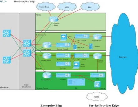
The Enterprise Edge, shown in Figure 1-4, details the connections from the campus to the WAN and includes:
n E-commerce
n Internet connectivity
n Remote access
THE EVOLVING NET WORK MODEL
FIGURE 1-4 The Enterprise Edge
Frame Relay ATM PPP
WAN
Corporate Router
E-Commerce
Web
DMZ Firewall Internet Router
Database I DC
App Server Internal Router Internal Firewall
Internet
Internal Router Internal Firewall DMZ Firewall
Public Servers
Internet Router
Internet Caching
Internal Router Firewall VPN
Campus Backbone
Edge Distribution
Remote Access IDS Dial-In
THE EVOLVING NET WORK MODEL
The Service Provider Edge is just a list of the public networks that facilitate wide-area connectivity and include:
n Internet service provider (ISP)
n Public switched telephone network (PSTN)
n Frame Relay, ATM, and PPP
Figure 1-5 puts together the various pieces: Campus, Enterprise Edge, and Service Provider Edge. Security implemented on this model is described in the Cisco SAFE (Security Architecture for Enterprise) blueprint.
FIGURE 1-5
E-Mail I DC
The Enterprise Composite Model
DNS File & Print IDC
Frame Relay
Legacy
Directory Database I DC Edge
Distribution WAN
ATM
Corporate Router SERVER FARM
PPP
E-Commerce
Web
DMZ Firewall Internet Router
Database I DC
CAMPUS BACKBONE
Internal Router Internal Firewall
App Server
BUILDING DISTRIBUITION Internet
Internal Router Internal Firewall DMZ Firewall
Public Servers
Internet Router
Management BUILDING DISTRIBUITION BUILDING DISTRIBUITION
Internet
4 Floor
4th Floor 3rd Floor
2nd Floor 1st Floor
BUILDING ACCESS
3rd Floor 2nd Floor 1st Floor BUILDING ACCESS
4th Floor 3rd Floor 2nd Floor 1st Floor BUILDING ACCESS
Internal Router
th
Caching
Firewall VPN
PSTN
Remote Access IDS Dial-In
Enterprise Campus Enterprise Edge Service
THE EVOLVING NET WORK MODEL
SONA and IIN
Modern converged networks include different traffic types, each with unique requirements for security, QoS, transmission capacity, and delay. These include:
n Voice signaling and bearer
n Core application traffic, such as Enterprise Resource Planning
IIN describes an evolutionary vision of a network that integrates network and application functionality cooperatively and allows the network to be smart about how it handles traffic to minimize the footprint of applications. IIN is built on top of the Enterprise Composite Model and describes structures overlaid on to the Composite design as needed in three phases.
Phase 1, ―Integrated Transport,‖ describes a converged network, which is built along the lines of the Composite model and based on open standards. This is the phase that the industry has been transitioning to recently. The Cisco Integrated Services Routers (ISR) are an example of this trend.
Phase 2, ―Integrated Services,‖ attempts to virtualize resources, such as servers, storage, and network access. It is a move to an ―on-demand‖ model.
By ―virtualize,‖ Cisco means that the services are not associated with a particular device or location. Instead, many services can reside in one device to ease management, or many devices can provide one service that is more reliable.
An ISR brings together routing, switching, voice, security, and wire-less. It is an example of many services existing on one device. A load balancer, which makes many servers look like one, is an example of one service residing on many devices.
VRFs are an example of taking one resource and making it look like many. Some versions of IOS are capable of having a router present itself as many virtual router (VRF) instances, allowing your company to deliver different logical topologies on the same physical infrastructure. Server virtualization is another example. The classic example of taking one resource and making it appear to be many resources is the use of a virtual LAN (VLAN) and a virtual storage area network (VSAN). (ERP) or Customer Relationship Management (CRM)
n Database transactions
n Multicast multimedia
n Network management
n Other traffic, such as web pages, e-mail, and file transfer Cisco routers are able to implement filtering, compression, prioritiza-tion, and policing. Except for filtering, these capabilities are referred to collectively as QoS.
Note
The best way to meet capacity requirements is to have twice as much band-width as needed. Financial reality, however, usually requires QoS instead.
THE EVOLVING NET WORK MODEL
Virtualization provides flexibility in configuration and management.
Phase 3, ―Integrated Applications,‖ uses application-oriented network-ing (AON) to make the network application-aware and to allow the network to actively participate in service delivery.
An example of this Phase 3 IIN systems approach to service delivery is Network Admission Control (NAC). Before NAC, authentication, VLAN assignment, and anti-virus updates were separately managed. With NAC in place, the network is able to check the policy stance of a client and admit, deny, or remediate based on policies.
IIN allows the network to deconstruct packets, parse fields, and take actions based on the values it finds. An ISR equipped with an AON blade might be set up to route traffic from a business partner. The AON blade can
FIGURE 1-6 IIN and SONA
examine traffic, recognize the application, and rebuild XML files in memory. Corrupted XML fields might represent an attack (called schema
poisoning), so the AON blade can react by blocking that source from
further communication. In this example, routing, an awareness of the application data flow, and security are combined to allow the network to contribute to the success of the application.
Services-Oriented Network Architecture (SONA) applies the IIN ideal to Enterprise networks. SONA breaks down the IIN functions into three layers:
n Network Infrastructure—Hierarchical converged network and attached end systems.
n Interactive Services—Resources allocated to applications.
n Applications—Includes business policy and logic.
IIN Phases
Phase 3 – Integrated Applications
(―application aware‖)
SONA Framework Layers
Business Apps
Middleware
Collaboration Layer Application
Layer Collaboration Apps
Middleware
Interactive Services Layer
Application Networking Services
Infrastructure Services Phase 2 – Integrated Services (virtualized resources)
Infra-structure Layer
Network
THE EVOLVING NET WORK MODEL
IP Routing Protocols
Routing protocols are used to pass information about the structure of the network between routers. Cisco routers support the following IP routing protocols RIP (versions 1 and 2), IGRP, EIGRP, IS-IS, OSPF, and BGP. This section compares routing protocols and calls out key differences between them.
Information Source AD
OSPF (Open Shortest Path First)
IS-IS (Intermediate System to Intermediate System)
RIP (Routing Information Protocol)
ODR (On Demand Routing)
External EIGRP
Internal BGP
110
115
120
160
170
200
255
Administrative Distance
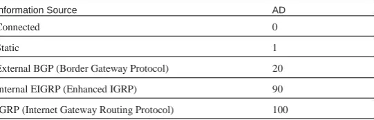
Cisco routers are capable of supporting several IP routing protocols concurrently. When identical prefixes are discovered from two or more separate sources, Administrative Distance (AD) is used to discriminate between the paths. AD is a poor choice of words; trustworthiness is a better name. Routers use paths with the lower AD.
Table 1-1 lists the default values for various routing protocols. Of course, there are several ways to change AD for a routing protocol or for a specific route.
TABLE 1-1 Routing Protocols and Their Default
Administrative Distance
Information Source AD
Unknown
Building the Routing Table
The router builds a routing table by ruling out invalid routes and considering the remaining advertisements. The procedure is:
1. For each route received, verify the next hop. If invalid, discard the route.
2. If multiple, valid routes are advertised by a routing protocol, choose the lowest metric.
3. Routes are identical if they advertise the same prefix and mask, so
Connected
Static
External BGP (Border Gateway Protocol)
Internal EIGRP (Enhanced IGRP)
IGRP (Internet Gateway Routing Protocol)
0
1
20
90
100
192.168.0.0/16 and 192.168.0.0/24 are separate paths and are each placed into the routing table.
THE EVOLVING NET WORK MODEL
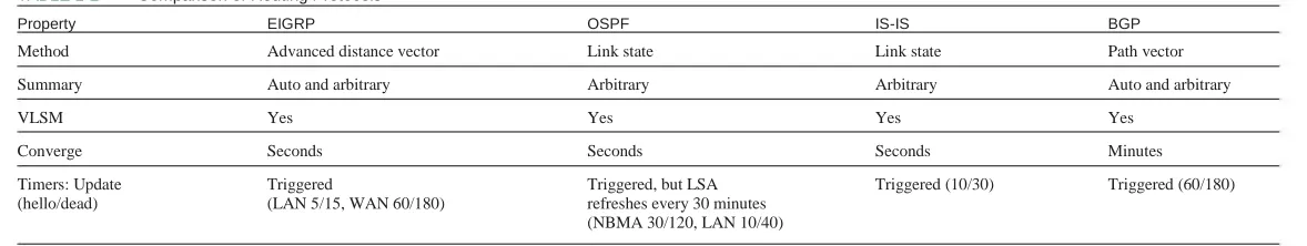
Comparing Routing Protocols
Two things should always be considered in choosing a routing protocol: fast convergence speed and support for VLSM. EIGRP, OSPF, and IS-IS meet these criteria. Although all three meet the minimum, there are still important distinctions, as described below:
n EIGRP is proprietary, but it is simple to configure and support.
n OSPF is an open standard, but it is difficult to implement and support.
n There are few books on IS-IS and even fewer engineers with experience who use it. IS-IS is therefore uncommon.
Table 1-2 compares routing protocols.
TABLE 1-2
Property
Comparison of Routing Protocols
EIGRP OSPF IS-IS BGP
Method
Summary
VLSM
Converge
Timers: Update (hello/dead)
Advanced distance vector
Auto and arbitrary
Yes
Seconds
Triggered
(LAN 5/15, WAN 60/180)
Link state
Arbitrary
Yes
Seconds
Triggered, but LSA refreshes every 30 minutes (NBMA 30/120, LAN 10/40)
Link state
Arbitrary
Yes
Seconds
Triggered (10/30)
Path vector
Auto and arbitrary
Yes
Minutes
CHAPTER 2
EIGRP
Enhanced Interior Gateway Routing Protocol (EIGRP) is a Cisco proprietary classless routing protocol that uses a complex metric based on bandwidth and delay. The following are some features of EIGRP:
n Fast convergence
n Support for VLSM
n Partial updates conserve network bandwidth
n Support for IP, AppleTalk, and IPX
n Support for all layer 2 (data link layer) protocols and topologies
n Sophisticated metric that supports unequal-metric proportional
n Diffusing Update Algorithm (DUAL)—Determines the best loop-free route
n Protocol-independent modules (PDM)—Modules are ―plug-ins‖ for IP, IPX, and AppleTalk versions of EIGRP
EIGRP uses three tables:
n The neighbor table is built from EIGRP hellos and used for reliable delivery.
n The topology table contains EIGRP routing information for best paths and loop-free alternatives.
n EIGRP places best routes from its topology table into the common load-balancing
n Use of multicasts (and unicasts where appropriate) instead of
routing table.
broadcasts
n Support for authentication
EIGRP Messages
EIGRP uses various message types to initiate and maintain neighbor relationships, and to maintain an accurate routing table. It is designed to conserve bandwidth and router resources by sending messages only when needed, and only to those neighbors that need to receive them.
EIGRP Overview
EIGRP’s function is controlled by four key technologies:
n Neighbor discovery and maintenance—Uses periodic hello messages
EIGRP
Packet Types
EIGRP uses five packet types:
n Hello—Identifies neighbors and serves as a keepalive mechanism
n Update—Reliably sends route information
n Query—Reliably requests specific route information
n Reply—Reliably responds to a query
n ACK—Acknowledgment
Step 1.
Step 2.
Step 3.
Step 4.
Step 5.
Router A sends out a hello.
Router B sends back a hello and an update. The update contains routing information.
Router A acknowledges the update. Router A sends its update. Router B acknowledges.
EIGRP is reliable, but hellos and ACKs are not acknowledged. The acknowledgement to a query is a reply.
If a reliable packet is not acknowledged, EIGRP periodically retrans-mits the packet to the nonresponding neighbor as a unicast. EIGRP has a window size of one, so no other traffic is sent to this neighbor until it responds. After 16 unacknowledged retransmissions, the neighbor is removed from the neighbor table.
Once two routers are EIGRP neighbors, they use hellos between them as keepalives. Additional route information is sent only if a route is lost or a new route is discovered. A neighbor is considered lost if no hello is received within three hello periods (called the hold time). The default hello/hold timers are as follows:
n 5 seconds/15 seconds for multipoint circuits with bandwidth greater than T1 and for point-to-point media
n 60 seconds/180 seconds for multipoint circuits with bandwidth less than or equal to T1
The exchange process can be viewed using debug ip eigrp packets,
and the update process can be seen using debug ip eigrp. The neighbor table can be seen with the command show ip eigrp neighbors.
Neighbor Discovery and Route Exchange
EIGRP
EIGRP Route Selection
An EIGRP router receives advertisements from each neighbor that lists the advertised distance (AD) and feasible distance (FD) to a route. The
AD is the metric from the neighbor to the network. FD is the metric from this router, through the neighbor, to the network.
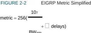
FIGURE 2-2 EIGRP Metric Simplified
107
metric 256(
delays)BWmin
If default k values are used, this works out to be 256 (BW + cumulative delay).
Bandwidth is the largest contributor to the metric. The delay value allows us to choose a more direct path when bandwidth is equivalent.
The EIGRP metric is 256 times the IGRP metric. The two automati-cally redistribute and algorithmiautomati-cally adjust metrics if they are config-ured on the same router for the same autonomous system.
EIGRP Metric
The EIGRP metric is shown in Figure 2-1.
FIGURE 2-1
metric 256(k1
EIGRP Metric
k5107k 2 BWmin k 3
delays)() reliability k 4BWmin 256 load
The k values are constants. Their default values are:
k1 = 1, k2 = 0, k3 = 1, k4 = 0, and k5 = 0. If k5 = 0, the final part of the equation (k5 / [rel + k4]) is ignored.
BWmin is the minimum bandwidth along the path—the choke point
bandwidth.
Delay values are associated with each interface. The sum of the delays (in tens of microseconds) is used in the equation.
Taking the default k values into account, the equation simplifies to the one shown in Figure 2-2.
Diffusing Update Algorithm (DUAL)
DUAL is the algorithm used by EIGRP to choose best paths by looking at AD and FD. The path with the lowest metric is called the successor
path. EIGRP paths with a lower AD than the FD of the successor path are guaranteed loop-free and called feasible successors. If the successor path is lost, the router can use the feasible successor immediately without risk of loops.
EIGRP
three minutes, the router becomes stuck in active (SIA). In that case, it resets the neighbor relationship with the neighbor that did not reply.
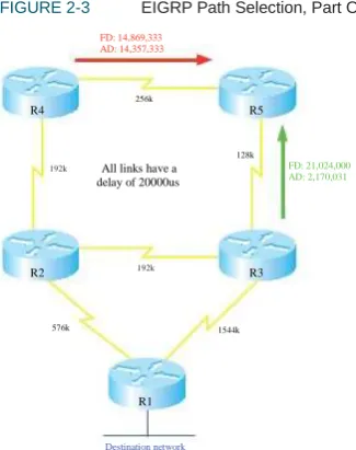
How does R3 choose its path? Figure 2-4 shows the path selection process for R3.
FIGURE 2-4 EIGRP Path Selection, Part Two
256k
Route Selection Example
The following diagrams show EIGRP advertisements to R3 and R5 about a destination network connected to R1. In Figure 2-3, R5 chooses R4 as the successor path because it offers the lowest feasible distance. The AD from R3 indicates that passing traffic through R3 will not loop, so R3 is a feasible successor.
FIGURE 2-3 EIGRP Path Selection, Part One
R2 192k R4
128k
R5
All links have a delay of 20000us
FD: 13,845,333 AD:4,956,444 192k
FD: 14,869,333 AD: 14,357,333
R3
576k
256k
1544k
FD:2,170,031 AD:0
R4
128k
R5
R1
Destination network All links have a
delay of 20000us
192k FD: 21,024,000
AD: 2,170,031
R2 192k R3
576k 1544k
R1 will be its successor because it has the lowest metric. However, no feasible successor exists because R2’s AD is greater than the successor path metric. If the direct path to R1 is lost, then R3 has to query its neighbors to discover an alternative path. It must wait to hear back from R2 and R5, and will ultimately decide that R2 is the new successor.
R1
EIGRP
Basic EIGRP Configuration
EIGRP is configured by entering router configuration mode and identi-fying the networks within which it should run. When setting up EIGRP, an autonomous system number must be used (7 is used in the example). Autonomous system numbers must agree for two routers to form a neighbor relationship and to exchange routes.
Router(config)#router eigrp 7
Router(config-router)#network 192.168.1.0
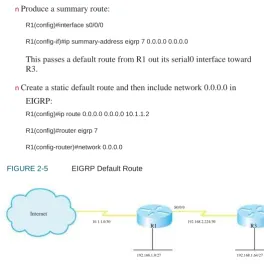
n Produce a summary route:
R1(config)#interface s0/0/0
R1(config-if)#ip summary-address eigrp 7 0.0.0.0 0.0.0.0
This passes a default route from R1 out its serial0 interface toward R3.
n Create a static default route and then include network 0.0.0.0 in EIGRP:
R1(config)#ip route 0.0.0.0 0.0.0.0 10.1.1.2
R1(config)#router eigrp 7
R1(config-router)#network 0.0.0.0
The wildcard mask option can be used with the network command to more precisely identify EIGRP interfaces. For instance, if a router has two interfaces—fa0/0 (192.168.1.1/27) and fa0/1 (192.168.1.33/27)—and needs to run only EIGRP on fa0/0, the following command can be used:
Router(config-router)#network 192.168.1.0 0.0.0.1
FIGURE 2-5 EIGRP Default Route
In this command, a wildcard mask of 0.0.0.1 matches only two IP addresses in network 192.168.1.0–192.168.1.0 and 192.168.1.1. Therefore, only interface fa0/0 is included in EIGRP routing.
S0/0/0
Internet
10.1.1.0/30
R1 192.168.2.224/30 R3
Creating an EIGRP Default Route
Figure 2-5 shows a simple two-router network. You can configure EIGRP on R1 to advertise a default route to R3 in three ways:
n R1 can specify a default network:
R1(config)#ip default-network 10.0.0.0
192.168.1.0/27 192.168.1.64/27
EIGRP
Troubleshooting EIGRP
The most straightforward way to troubleshoot EIGRP is to inspect the routing table—show ip route. To filter the routing table and show only the routes learned from EIGRP, use the show ip route eigrp command.
The show ip protocols command verifies autonomous system, timer
values, identified networks, and EIGRP neighbors (routing information sources).
The command show ip eigrp topology shows the EIGRP topology table and identifies successors and feasible successors. Use show ip eigrp
neighbors to verify that the correct routers are neighbors, and use show
ip eigrp traffic to show the amount and types of EIGRP messages.
Summaries can be produced manually on any interface. When a summary is produced, a matching route to null0 also becomes active as a loop prevention mechanism. Configure a summary route out a partic-ular interface using the ip summary-address eigrp autonomous_system
command. The following example advertises a default route out FastEthernet0/1 and the summary route 172.16.104.0/22 out Serial0/0/0 for EIGRP AS 7.
Router(config)#int fa0/1
Router(config-if)#ip summary-address eigrp 7 0.0.0.0 0.0.0.0 !
Router(config)#int s0/0/0
Router(config-if)#ip summary-address eigrp 7 172.16.104.0 255.255.252.0
Advanced EIGRP Configuration
EIGRP provides some ways to customize its operation, such as route summarization, unequal-metric load balancing, controlling the percent of interface bandwidth used, and authentication. This section describes how to configure these.
Load Balancing
EIGRP, like most IP routing protocols, automatically load balances over equal metric paths. What makes EIGRP unique is that you can configure it to proportionally load balance over unequal metric paths. The variance
command is used to configure load balancing over up to six loop-free paths with a metric lower than the product of the variance and the best metric. Figure 2-3, in the ―Route Selection Example‖ section, shows routers advertising a path to the network connected to R1.
By default, R5 uses the path through R4 because it offers the lowest metric (14,869,333). To set up unequal cost load balancing, assign a variance of 2 under the EIGRP process on R5. R5 multiplies the best metric of 14,869,333 by 2, to get 29,738,666. R5 then uses all loop-free
Summarization
EIGRP defaults to automatically summarizing at classful network boundaries. Automatic summarization is usually disabled using the following command:
EIGRP
paths with a metric less than 29,738,666, which includes the path through R3. By default, R5 load balances over these paths, sending traffic along each path in proportion to its metric.
R5(config)#router eigrp 7
R5(config-router)#variance 2
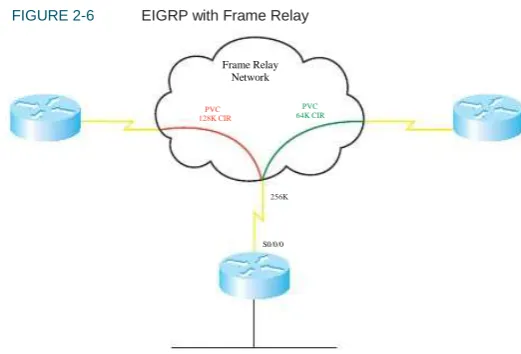
PVC 128K CIR
FIGURE 2-6 EIGRP with Frame Relay
Frame Relay Network
PVC 64K CIR
By default, EIGRP limits itself to bursting to half the link bandwidth. This limit is configurable per interface using the ip bandwidth-percent
command. The following example assumes EIGRP AS 7 and limits EIGRP to one quarter of the link bandwidth:
Router(config)#int s0/0/0
Router(config-if)#ip bandwidth-percent eigrp 7 25
S0/0/0
The real issue with WAN links is that the router assumes that each link has 1544 kbps bandwidth. If interface Serial0/0/0 is attached to a 128 k fractional T1, EIGRP assumes it can burst to 768 k and could over-whelm the line. This is rectified by correctly identifying link band-width.
Router (config)#int serial 0/0/0
Router (config-if)#bandwidth 128
Figure 2-6 shows a situation in which these techniques can be combined—Frame Relay.
In this example, R1 has a 256 kbps connection to the Frame Relay network and two permanent virtual circuits (PVCs) with committed information rates (CIR) of 128 Kpbs and 64 Kbps. EIGRP divides the interface bandwidth evenly between the number of neighbors on that interface. What value should be used for the interface bandwidth in this case? The usual suggestion is to use the CIR, but the two PVCs have different CIRs. You could use the bandwidth-percent command to allow SNMP reporting of the true bandwidth value, while adjusting the inter-face burst rate to 25 percent, or 64 kbps.
256K
EIGRP
R1(config)#int serial 0/0/0 R1 (config-if)#bandwidth 256
R1 (config-if)#ip bandwidth-percent eigrp 7 25
To configure EIGRP authentication, follow these steps:
Step 1.
Step 2.
Step 3.
Step 4.
Configure a key chain to group the keys. Configure a key within that key chain.
Configure the password or authentication string for that key. Repeat Steps 2 and 3 to add more keys if desired.
Optionally configure a lifetime for the keys within that key chain. If you do this, be sure that the time is synchronized between the two routers.
Enable authentication and assign a key chain to an inter-face.
Designate MD5 as the type of authentication. A better solution is to use subinterfaces and identify bandwidth
sepa-rately. In the following example, s0/0/0.1 bursts to 64 k, and s0/0/0.2 bursts to 32 k, using EIGRP’s default value of half the bandwidth.
R1(config)#int serial 0/0/0.1 R1 (config-if)#bandwidth 128 !
R1(config)#int serial 0/0/0.2
R1 (config-if)#bandwidth 64 Step 5.
Step 6.
In cases where the hub interface bandwidth is oversubscribed, it may be necessary to set bandwidth for each subinterface arbitrarily low, and then specify an EIGRP bandwidth percent value over 100 in order to allow EIGRP to use half the PVC bandwidth.
EIGRP Authentication
By default, no authentication is used for any routing protocol. Some protocols, such as RIPv2, IS-IS, and OSPF, can be configured to do simple password authentication between neighboring routers. In this type of authentication, a clear-text password is used. EIGRP does not support simple authentication. However, it can be configured to authenticate each packet exchanged, using an MD5 hash. This is more secure than clear text, as only the message digest is exchanged, not the password.
EIGRP authenticates each of its packets by including the hash in each one. This helps verify the source of each routing update.
Example 2-1 shows a router configured with EIGRP authentication. It shows configuring a lifetime for packets sent using key 1 that starts at 10:15 and lasts for 300 seconds. It also shows configuring a lifetime for packets received using key 1 that starts at 10:00 and lasts until 10:05.
EXAMPLE 2-1 Configuring EIGRP Authentication
Router(config)#key chain RTR_Auth Router(config-keychain)#key 1
Router(config-keychain-key)#key-string mykey Router(config-keychain-key)#send-lifetime 10:15:00 300 Router(config-keychain-key)#accept-lifetime 10:00:00 10:05:00 !
Router(config)#interface s0/0/0
Router(config-if)#ip authentication mode eigrp 10 md5
EIGRP
Verify your configuration with the show ip eigrp neighbors command, as no neighbor relationship will be formed if authentication fails. Using
the debug eigrp packets command should show packets containing
authentication information sent and received, and it will allow you to troubleshoot configuration issues.
Routers use SIA-Queries and SIA-Replies to prevent loss of a neighbor unnecessarily during SIA conditions. A router sends its neighbor a SIA-Query after no reply to a normal query. If the neighbor responds with a SIA-Reply, then the router does not terminate the neighbor relationship after three minutes, because it knows the neighbor is available.
Graceful shutdown is another feature that speeds network convergence.
Whenever the EIGRP process is shut down, the router sends a ―goodbye‖ message to its neighbors. The neighbors can then immedi-ately recalculate any paths that used the router as the next hop, rather than waiting for the hold timer to expire.
EIGRP Scalability
Four factors influence EIGRP’s scalability:
n The number of routes that must be exchanged
n The number of routers that must know of a topology change
n The number of alternate routes to a network
n The number of hops from one end of the network to the other
To improve scalability, summarize routes when possible, try to have a network depth of no more than seven hops, and limit the scope of EIGRP queries.
Stub routing is one way to limit queries. A stub router is one that is
connected to no more than two neighbors and should never be a transit router. When a router is configured as an EIGRP stub, it notifies its neighbors. The neighbors then do not query that router for a lost route. Under router configuration mode, use the command eigrp stub
[receive-only|connected|static|summary]. An EIGRP stub router still
CHAPTER 3
OSPF
OSPF Overview
OSPF is an open-standard, classless routing protocol that converges quickly and uses cost as a metric (Cisco IOS automatically associates cost with bandwidth).
OSPF is a link-state routing protocol and uses Dijkstra’s Shortest Path First (SPF) algorithm to determine its best path to each network. The first responsibility of a link-state router is to create a database that reflects the structure of the network. Link state routing protocols learn more information on the structure of the network than other routing protocols, and thus are able to make more informed routing decisions.
OSPF routers exchange hellos with each neighbor, learning Router ID (RID) and cost. Neighbor information is kept in the adjacency database.
The router then constructs the appropriate Link State Advertisements (LSA), which include information such as the RIDs of, and cost to, each neighbor. Each router in the routing domain shares its LSAs with all other routers. Each router keeps the complete set of LSAs in a table—the Link State Database (LSDB).
Each router runs the SPF algorithm to compute best paths. It then submits these paths for inclusion in the routing table, or forwarding database.
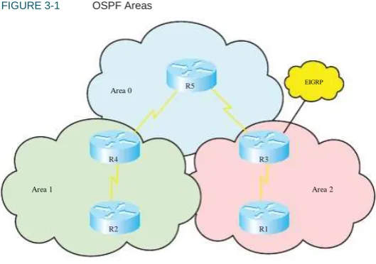
OSPF Network Structure
OSPF routing domains are broken up into areas. An OSPF network must contain an area 0, and may contain other areas. The SPF algo-rithm runs within an area, and inter-area routes are passed between areas. A two-level hierarchy to OSPF areas exists; area 0 is designed as a transit area, and other areas should be attached directly to area 0 and only to area 0. The link-state database must be identical for each router in an area. OSPF areas typically contain a maximum of 50–100 routers, depending on network volatility. Figure 3-1 shows a network of five routers that has been divided into three areas: area 0, area 1, and area 2.
FIGURE 3-1 OSPF Areas
Area 0 R5
EIGRP
R4
Area 1
R3
Area 2
OSPF
Dividing an OSPF network into areas does the following:
n Minimizes the number of routing table entries.
n Contains LSA flooding to a reasonable area.
n Minimizes the impact of a topology change.
n Enforces the concept of a hierarchical network design.
FIGURE 3-2 OSPF Cost Formula
Cost= 100 Mbps
Bandwidth
OSPF defines router roles as well. One router can have multiple roles.
n An internal router has all interfaces in one area. In Figure 3-1, R1, R2, and R5 are all internal area routers.
n Backbone routers have at least one interface assigned to area 0.
The default formula doesn’t differentiate between interfaces with speeds faster than 100 Mbps. It assigns the same cost to a Fast Ethernet interface and a Gigabit Ethernet interface, for example. In such cases, the cost formula can be adjusted using the auto-cost command under the OSPF routing process. Values for bandwidth (in kbps) up to 4,294,967 are permitted (1 Gbps is shown in the following line):
Router(config-router)#auto-cost reference-bandwidth 1000
R3, R4, and R5 are backbone routers.
n An Area Border Router (ABR) has interfaces in two or more areas. In Figure 3-1, R3 and R4 are ABRs.
n An Autonomous System Boundary Router (ASBR) has interfaces
The cost can also be manually assigned under the interface configuration mode. The cost is a 16-bit number, so it can be any value from 1 to 65,535.
Router(config-router)#ip ospf cost 27
inside and outside the OSPF routing domain. In Figure 3-1, R3 also functions as an ASBR because it has an interface in an
EIGRP routing domain.
LSAs
Each router maintains a database of the latest received LSAs. Each LSA is numbered with a sequence number, and a timer is run to age out old LSAs.
When a LSA is received, it’s compared to the LSDB. If it is new, it is added to the database and the SPF algorithm is run. If it is from a Router ID that is already in the database, then the sequence number is compared, and older LSAs are discarded. If it is a new LSA, it is incorporated in the database, and the SPF algorithm is run. If it is an older LSA, the newer LSA in memory is sent back to whoever sent the old one.
OSPF Metric
OSPF
OSPF sequence numbers are 32 bits. The first legal sequence number is 0x80000001. Larger numbers are more recent. The sequence number changes only under two conditions:
n The LSA changes because a route is added or deleted.
n The LSA ages out (LSAs are updated every half hour, even if
[warningonly][ignore-time minutes] [ignore-count number]
[reset-time minutes]. The meaning of the keywords of this command are:
n Maximum-number—The threshold. This is the most nonlocal
LSAs that the router can maintain in its LSDB.
n Threshold-percentage—A warning message is sent when this
nothing changes).
The command show ip ospf database shows the age (in seconds) and sequence number for each RID.
percentage of the threshold number is reached. The default is 75 percent.
n Warningonly—This causes the router to send only a warning; it
does not enter the ignore state.
n Ignore-time minutes—Specifies the length of time to stay in the
LSDB Overload Protection
Because each router sends an LSA for each link, routers in large networks may receive—and must process—numerous LSAs. This can tax the router’s CPU and memory resources, and adversely affect its other functions. You can protect your router by configuring OSPF LSDB overload protection. LDSB overload protection monitors the number of LSAs received and placed into the LSDB. If the specified threshold is exceeded for one minute, the router enters the ―ignore‖ state by dropping all adjacencies and clearing the OSPF database. The router resumes OSPF operations after things have been normal for a specified period. Be careful when using this command, as it disrupts routing when invoked.
Configure LSDB overload protection with the OSPF router process command max-lsa maximum-number [threshold-percentage]
ignore state. The default is five minutes.
n Ignore-count number—Specifies the maximum number of times a
router can go into the ignore state. When this number is exceeded, OSPF processing stays down and must be manually restarted. The default is five times.
n Reset-time minutes—The length of time to stay in the ignore
state. The default is ten minutes.
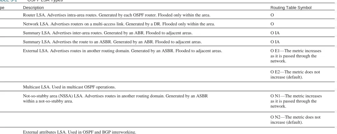
LSA Types
OSPF
TABLE 3-1
Type
OSPF LSA Types
Description Routing Table Symbol
1
2
3
4
5
Router LSA. Advertises intra-area routes. Generated by each OSPF router. Flooded only within the area.
Network LSA. Advertises routers on a multi-access link. Generated by a DR. Flooded only within the area.
Summary LSA. Advertises inter-area routes. Generated by an ABR. Flooded to adjacent areas.
Summary LSA. Advertises the route to an ASBR. Generated by an ABR. Flooded to adjacent areas.
External LSA. Advertises routes in another routing domain. Generated by an ASBR. Flooded to adjacent areas.
O
O
O IA
O IA
O E1—The metric increases as it is passed through the network.
O E2—The metric does not increase (default).
6
7
Multicast LSA. Used in multicast OSPF operations.
Not-so-stubby area (NSSA) LSA. Advertises routes in another routing domain. Generated by an ASBR within a not-so-stubby area.
O N1—The metric increases as it is passed through the network.
O N2—The metric does not increase (default).
8
9, 10, 11
External attributes LSA. Used in OSPF and BGP interworking.
OSPF
OSPF Operation
OSPF uses several different message types to establish and maintain its neighbor relationships, and to maintain correct routing information. When preparing for the exam, be sure you understand each OSPF packet type, and the OSPF neighbor establishment procedure.
OSPF traffic is multicast to either of two addresses: 224.0.0.5 for all OSPF routers or 224.0.0.6 for all OSPF DRs.
OSPF Neighbor Relationships
OSPF routers send out periodic multicast packets to introduce them-selves to other routers on a link. They become neighbors when they see their own router ID included in the Neighbor field of the hello from another router. Seeing this tells each router that they have bidirectional communication. In addition, two routers must be on a common subnet for a neighbor relationship to be formed. (Virtual links are sometimes an exception to this rule.)
Certain parameters within the OSPF hellos must also match in order for two routers to become neighbors. They include:
n Hello/dead timers
n Area ID
n Authentication type and password
n Stub area flag
OSPF Packets
OSPF uses five packet types. It does not use UDP or TCP for transmit-ting its packets. Instead, it runs directly over IP (IP protocol 89) using an OSPF header. One field in this header identifies the type of packet being carried. The five OSPF packet types are:
n Hello—Identifies neighbors and serves as a keepalive.
n Link State Request (LSR)—A request for an Link State Update
(LSU). Contains the type of LSU requested and the ID of the router requesting it.
n Database Description (DBD)—A summary of the LSDB,
includ-ing the RID and sequence number of each LSA in the LSDB.
n Link State Update (LSU)—Contains a full LSA entry. An LSA
includes topology information; for example, the RID of this router and the RID and cost to each neighbor. One LSU can contain multiple LSAs.
n Link State Acknowledgment (LSAck)—Acknowledges all other
OSPF packets (except hellos).
OSPF
Hellos also serve as keepalives. A neighbor is considered lost if no Hello is received within four Hello periods (called the dead time). The default hello/dead timers are as follows:
n 10 seconds/40 seconds for LAN and point-to-point interfaces
n 30 seconds/120 seconds for nonbroadcast multiaccess (NBMA)
Step 5.
Step 6.
Exchange state—Routers exchange DBDs listing the
LSAs in their LSD by RID and sequence number.
Loading state—Each router compares the DBD received
to the contents of its LS database. It then sends a LSR for missing or outdated LSAs. Each router responds to its neighbor’s LSR with a Link State Update. Each LSU is acknowledged.
Full state—The LSDB has been synchronized with the
adjacent neighbor. interfaces
Step 7.
Establishing Neighbors and Exchanging
Routes
The process of neighbor establishment and route exchange between two OSPF routers is as follows:
Step 1.
Step 2.
Step 3.
Basic OSPF Configuration
OSPF is configured by entering router configuration mode and identify-ing the range of interface addresses on which it should run and the areas they are in. When setting up OSPF, a process ID must be used (8 is used in the example), but the process ID does not have to agree on different OSPF devices for them to exchange information. The network statement uses a wildcard mask and can specify any range from a single address to all addresses. Unlike EIGRP, the wildcard mask is not optional. The following example shows a router configured as an ABR. Interfaces falling with the 192.168.1.0 network are placed in area 0, and interfaces falling within the 172.16.1.0 network are placed in area 1.
Router(config)#router ospf 8
Router(config-router)#network 192.168.1.0 0.0.0.255 area 0
Router(config-router)#network 172.16.1.0 0.0.0.255 area 1
Down state—OSPF process not yet started, so no hellos
sent.
Init state—Router sends hello packets out all OSPF
interfaces.
Two-way state—Router receives a hello from another
router that contains its own router ID in the neighbor list. All other required elements match, so routers can become neighbors.
Exstart state—If routers become adjacent (exchange
routes), they determine who will start the exchange process.
OSPF
Router ID
The SPF algorithm is used to map the shortest path between a series of nodes. This causes an issue with IP, because an IP router is not identi-fied by a single IP address—its interfaces are. For this reason, a single IP address is designated as the ―name‖ of the router—the RID.
By default, the RID is the highest loopback IP address. If no loopback addresses are configured, the RID is the highest IP address on an active interface when the OSPF process is started. The RID is selected when OSPF starts and—for reasons of stability—is not changed until OSPF restarts. The OSPF process can be restarted by rebooting or by using the command clear ip ospf process. Either choice affects routing in your network for a period of time and should be used only with caution.
A loopback interface is a virtual interface, so it is more stable than a physical interface for RID use. A loopback address is configured by creating an interface and assigning an IP address.
Router(config)#interface loopback0
Router(config-if)#ip address 10.0.0.1 255.255.255.255
Troubleshooting OSPF
The neighbor initialization process can be viewed using the debug ip
ospf adjacencies command. The neighbor table can be seen with show
ip ospf neighbors, which also identifies adjacency status, and reveals
the designated router and backup designated router. Use the debug ip
ospf packet command to view all OSPF packets in real time.
Often, the first place OSPF issues are noticed is when inspecting the routing table—show ip route. To filter the routing table and show only the routes learned from OSPF, use show ip route ospf.
The command show ip protocols offers a wealth of information for any routing protocol issue. Use this command to verify parameters, timer values, identified networks, and OSPF neighbors (routing infor-mation sources).
Use show ip ospf to verify the RID, timers, and counters. Because
wildcard masks sometimes incorrectly group interfaces to areas, another good place to check is show ip ospf interface. This shows the interfaces on which OSPF runs and their current correct assigned area.
The loopback address does not have to be included in the OSPF routing process, but if you advertise it, you are able to ping or trace to it. This can help in troubleshooting.
A way to override the default RID selection is to statically assign it using the OSPF router-id command.
Router(config)#router ospf 8
Router(config-router)#router-id 10.0.0.1
OSPF Network Types
OSPF
represent the entire segment. Point-to-point links fit the SPF model perfectly and don’t need any special modeling method. On a point-to-point link, no DR is elected and all traffic is multicast to 224.0.0.5.
OSPF supports five network types:
n NBMA—Default for multipoint serial interfaces. RFC-compliant
Designated Routers
On a multiaccess link, one of the routers is elected as a DR and another as a backup DR (BDR). All other routers on that link become adjacent only to the DR and BDR, not to each other (they stop at the two-way state). The DR is responsible for creating and flooding a network LSA (type 2) advertising the multiaccess link. NonDR (DROTHER) routers communicate with DRs using the IP address 224.0.0.6. The DRs use IP address 224.0.0.5 to pass information to other routers.
The DR and BDR are elected as follows:
Step 1.
mode that uses DRs and requires manual neighbor configuration.
n Point-to–multipoint (P2MP)—Doesn’t use DRs so adjacencies
increase logarithmically with routers. Resilient RFC compliant mode that automatically discovers neighbors.
n Point-to-multipoint nonbroadcast (P2MNB)—Proprietary mode
that is used on Layer 2 facilities where dynamic neighbor discov-ery is not supported. Requires manual neighbor configuration.
n Broadcast—Default mode for LANs. Uses DRs and automatic
A router starting the OSPF process listens for OSPF hellos. If none are heard within the dead time, it declares itself the DR.
If hellos from any other routers are heard, the router with the highest OSPF priority is elected DR, and the election process starts again for BDR. A priority of zero removes a router from the election.
If two or more routers have the same OSPF priority, the router with the highest RID is elected DR, and the election process starts again for BDR.
Step 2.
neighbor discovery. Proprietary when used on WAN interface.
n Point-to–point (P2P)—Proprietary mode that discovers neighbors
and doesn’t require a DR.
If the default interface type is unsatisfactory, you can statically configure it with the command ip ospf network under interface configuration mode:
Router(config-if)#ip ospf network point-to-multipoint
Step 3.
When using the NBMA or P2MP nonbroadcast mode, neighbors must be manually defined under the routing process:
Router(config-router)#neighbor 172.16.0.1
After a DR is elected, elections do not take place again unless the DR or BDR are lost. Because of this, the DR is sometimes the first device that comes online with a nonzero priority.
OSPF
zero means that a router cannot act as DR or BDR; it can be a DROTHER only. Priority can be set with the ip ospf priority
command in interface configuration mode.
Router(config)#int fa 0/1
Router(config-if)#ip ospf priority 2
n Full-mesh environments can be configured using the physical interface, but often logical interfaces are used to take advantage of the other benefits of subinterfaces.
n It may be necessary to statically identify neighbor IP addresses.
Nonbroadcast Multiaccess (NBMA)
Networks
Routing protocols assume that multiaccess links support broadcast and have full-mesh connectivity from any device to any device. In terms of OSPF, this means the following:
n All Frame Relay or ATM maps should include the broadcast
Advanced OSPF Configuration
OSPF provides many different ways to customize its operation to fit your network needs. This section discusses route summarization, default routes, stub areas, and virtual links.
OSPF Summarization
Summarization helps all routing protocols scale to larger networks, but OSPF especially benefits because its processes tax the memory and CPU resources of the routers. The SPF algorithm consumes all CPU resources when it runs. Summarization prevents topology changes from being passed outside an area and thus saves routers in other areas from having to run the SPF algorithm. OSPF’s multiple databases use more memory the larger they are. Summarization decreases the number of routes exchanged, and thus the size of the databases. OSPF can produce summaries within a classful network (VLSM) or summaries of blocks of classful networks (CIDR). There are two types of summarizations: attribute.
n The DR and BDR should have full virtual circuit connectivity to all other devices.
n Hub-and-spoke environments should either configure the DR as the hub or use point-to-point subinterfaces, which require no DR.
OSPF
n Inter-area route summarizations are created on the ABR under
the OSPF routing process using the area range command. The following command advertises 172.16.0.0/12 from area 1:
Router(config-router)#area 1 range 172.16.0.0 255.240.0.0
Alternatively, a default summary route can also be produced using the
summary-address command or the area range command. These
commands cause the router to advertise a default route pointing to itself.
Reducing routing information in non-backbone areas is a common requirement because these routers are typically the most vulnerable in terms of processor and speed, and the links that connect them usually have the least bandwidth. A specific concern is that an area will be overwhelmed by external routing information.
n External route summarization is done on an ASBR using the
summary-address command under the OSPF routing process. The following example summarizes a range of external routes to 192.168.0.0/16 and injects a single route into OSPF.
Router(config-router)#summary-address 192.168.0.0 255.255.0.0
Stub and Not-So-Stubby Areas
Another way to reduce the route information advertised is to make an area a stub area. Configuring an area as a stub area forces its ABR to drop all external (type 5) routes and replaces them with a default route. To limit routing information even more, an area can be made totally stubby using the no-summary keyword on the ABR only. In that case, all interarea and external routes are dropped by the ABR and replaced by a default route. The default route starts with a cost of 1; to change it, use the area default-cost command. The example that follows shows area 2 configured as a totally stubby area, and the default route injected with a cost of 5:
Router(config-router)#area 2 stub no-summary
Router(config-router)#area 2 default-cost 5
Creating a Default Route
The default route is a special type of summarization; it summarizes all networks down to one route announcement. This provides the ultimate benefit of summarization by reducing routing information to a minimum. There are several ways to use the router IOS to place a default route into OSPF.
The best-known way to produce an OSPF default is to use the
default-information command under the OSPF routing process. This command,
without the keyword always, readvertises a default route learned from another source into OSPF. If the always keyword is present, OSPF advertises a default even if one does not already exist in the routing table. The metric keyword sets the starting metric for this route.
Router(config-router)#default-information originate [always] [metric metric]
OSPF
n Stub areas can’t include a virtual link.
n Stub areas can’t include an ASBR.
n Stubbiness must be configured on all routers in the area.
Area 0
Area 1
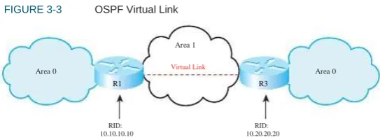
FIGURE 3-3 OSPF Virtual Link
Virtual Link Area 0
R3
Another kind of stub area is a not-so-stubby area (NSSA). NSSA is like a stub or totally stub area, but allows an ASBR within the area. External routes are advertised as type 7 routes by the ASBR. The ABR converts them to type 5 external routes when it advertises them into adjacent areas. NSSA is configured with the area nssa command under the OSPF routing process. The no-summary keyword on the ABR configures the area as a totally NSSA area; this is a Cisco proprietary feature. By default, the ABR does not inject a default route back into an NSSA area. Use the default-information-originate keyword on the ABR or ASBR to create this route.
Router(config-router)#area 7 nssa [no-summary] information-originate]
R1
RID: 10.10.10.10
RID: 10.20.20.20
Area 1 is the transit area for the virtual link. Configure each end of a virtual link on the ABRs of the transit area with the command area
area-number virtual-link router-id. Each end of the link is identified
by its RID. The area listed in the command is the transit area, not the area being joined by the link. The configuration for R1 is:
R1(config)#router ospf 1
R1(config-router)#area 1 virtual-link 10.20.20.20
The configuration for R2 is:
Configuring Virtual Links
OSPF requires that all areas be connected to area 0 and that area 0 must be contiguous. When this is not possible, you can use a virtual link to bridge across an intermediate area. Figure 3-3 shows a virtual link connecting two portions of area 0.
R2(config)#router ospf 1
R2(config-router)#area 1 virtual-link 10.10.10.10
Verify that the virtual link is up with the show ip ospf virtual-links
command. Additionally, virtual interfaces are treated as actual interfaces by the OSPF process, and thus, their status can be verified with the
OSPF
Configuring OSPF
Authentication
For security purposes, you can configure OSPF to authenticate every OSPF packet and the source of every OSPF routing update. By default, the router does no authentication. OSPF supports three types of authentication:
n Null authentication for a link that does not use authentication at all
n Simple (plain text) authentication
n MD5 authentication
The next example shows the same router configured for OSPF MD5 authentication for area 0, using a password of ―secure‖. Note that the commands are slightly different. The optional keyword message-digest
is required in two of the commands, and a key number must be speci-fied. Any neighbors reachable through the Gi0/1 interface must also be configured with the same key.
Router(config-router)#int gi0/1
Router(config-if)#ip ospf message-digest-key 2 md5 secure Router(config-if)#ip ospf authentication message-digest Router(config-if)#!
Router(config-if)#router ospf 1
Router(config-router)#area 0 authentication message-digest
The following example shows a router configured for simple password authentication in OSPF area 1, using a password of ―simple‖. Note that authentication commands are necessary both under the OSPF process and the interface configuration. All OSPF neighbors reachable through an interface configured for authentication must use the same password. You can, however, use different passwords for different interfaces.
Router(config)#int gi0/0
Router(config-if)#ip ospf authentication-key simple Router(config-if)#ip ospf authentication Router(config-if)#!
Router(config-if)#router ospf 1
CHAPTER 4
IS-IS
Intermediate System-to-Intermediate System (IS-IS) is a link state
routing protocol that is part of the OSI family of protocols. Like OSPF, it uses Dijkstra’s SPF algorithm to choose routes. IS-IS is a classless interior gateway protocol that uses router resources efficiently and scales to large networks, such as large Internet service providers (ISP).
Table 4-1 lists some IS-IS terms, acronyms, and their meanings.
TABLE 4-1
Term
IS-IS Acronyms
Acronym Description
Circuit ID
Complete Sequence Number PDU
Connectionless Network Protocol
Connectionless Network Services
End System
Intermediate System
Intermediate System hello
IS to IS hello
Link State Database
Link State PDU
Network Entity Title
CSNP
CLNP
CNLS
ES
IS
ISH
IIH
LSDB
LSP
NET
Identifies a physical interface on the router.
A summary of a router’s complete LSDB.
OSI protocol used to provide the connectionless services.
OSI data delivery service that provides best-effort delivery.
A host, such as a computer.
The OSI name for a router.
Sent by routers to hosts.
Hellos exchanged between routers. Seperate level 1 and level 2 IIHs exist.
A database containing all the LSAs the router knows about, and it keeps a separate LSDB for each area it belongs to.
A routing update.
A router’s NSAP. The last byte of a NET is always zero.
IS-IS
TABLE 4-1
Term
IS-IS Acronyms Continued
Acronym Description
Network Service Access Point
NSAP Selector
Protocol Data Unit
Partial Route Calculation
Partial Sequence Number PDU
Sequence Number Protocol Data Unit
Subnetwork Point of Attachment
Type Length Value
NSAP
NSEL
PDU
PRC
PSNP
SNP
SNPA
TLV
Address of a CLNS device. Addresses are assigned per device, not per interface as with IP.
The last byte of a NSAP address. Identifies the process on the device, such as routing.
A unit of data.
Used to determine end system and IP subnet reachability.
Used to acknowledge receipt of a CSNP and to request more information about a network contained in a CSNP.
An IS-IS packet that is sequenced and must be acknowledged. The sequence number helps a router maintain the most recent link state information.
Layer 2 identification for a router’s interface, such as MAC address or DLCI.
Fields in the IS-IS updates that contain IP subnet, authentication, and end-system information.
IS-IS Overview
Integrated IS-IS can carry IP network information, but does not use IP as its transport protocol. It uses OSI protocols CLNS and CLNP to deliver its updates. IS-IS sends its messages in PDUs. There are four IS-IS PDU types: Hello, LSP, PSNP, and CSNP.
Types of IS-IS Routers
IS-IS
Within an area, routers can be one of three types:
n Level 1 (L1) router—R1, R2, and R5 in the figure. Routes to
FIGURE 4-1 IS-IS Network Structure
networks only within the local area (intra-area routing). Uses a default route to the nearest Level 2 router for traffic bound outside the area. Keeps one LSDB for the local area. When routing, compares the area of the destination to its area. If they are the same, routes based on system ID. If not, sends traffic to Level 1-2 router.
n Level 2 (L2) router—R6 in the figure. Routes to networks in
Area 49.0001
R1 - L1
R2 - L1 R3 - L1-2
other areas (interarea routing). The routing is based on area ID. Keeps one LSDB for routing to other areas.
n Level 1-2 (L1-2) router—R3 and R4 in this figure. Acts as a
Area 49.0003 R6 - L2
gateway into and out of an area. Does Level 1 routing within the area and Level 2 routing between areas. Keeps two LSDB: one for the local area and one for interarea routing.
The IS-IS method of selecting routes can result in suboptimal routing between areas. To solve this, RFC 2966 introduces route leaking, which allows some L2 routes to be advertised (or leaked) into L1 areas.
Area 49.0002
R4 - L1-2
R5 - L1
NSAP Address Structure
IS-IS
n Area IDs vary from 1 to 13 bytes. Those that begin with 49 designate n Level 1-2 routers form Level 1 adjacencies with L1 routers in their private area addressing.
n The Cisco system ID must be exactly six bytes. MAC addresses or IP addresses padded with 0s are often used as system IDs.
n The NSEL is exactly one byte in size. A router always has a
own area, and Level 2 adjacencies with routers in other areas. (In Figure 4-1, R4 has a L1 adjacency with R5 and a L2 adjacency with R6.)
NSEL of 00.
Figure 4-2 shows the composition of an NSAP address.
FIGURE 4-2 IS-IS NSAP Address
IS-IS Network Types
IS-IS recognizes only broadcast and point-to-point links. In Frame Relay, multipoint interfaces must be fully meshed. Use point-to-point subinterfaces to avoid this.
On a broadcast network, IS-IS routers elect a Designated Intermediate System (DIS). The DIS is elected based on priority, with MAC address as the tie breaker (the lowest number wins for both priority and MAC address). Routers form adjacencies with the DIS and all other routers on the LAN. The DIS creates a pseudonode to represent the network and sends out an advertisement to represent the LAN. All routers advertise only an adjacency to the pseudonode. If the DIS fails, another is elected; no backup DIS exists. The DIS sends Hellos every 3.3 seconds; other routers send them every 10 seconds. The DIS also multi-casts a CSNP every 10 seconds.
No DIS exists on a point-to-point link. When an adjacency is first formed over the link, the routers exchange CSNPs. If one of the routers needs more information about a specific network, it sends a PSNP requesting that. After the initial exchange, LSPs are sent to describe link changes, and they are acknowledged with PSNPs. Hellos are sent every 10 seconds.
49.0234.0987.0000.2211.00
Area ID - 1 to 13
bytes long System ID - Must be exactly 6 bytes long NSEL – 1 byte
Adjacency Formation in IS-IS
IS-IS routers form adjacencies based on the level of IS routing they are doing and their area number. This is a CLNS adjacency and can be formed even if IP addresses don’t match.
n Level 1 routers form adjacencies only with L1 and L1-2 devices in their own area. (In Figure 4-1, R1 becomes adjacent with R2 and R3.)
IS-IS
Configuring IS-IS
The essential tasks to begin IS-IS routing are:
n Enable IS-IS on the router:
Router(config)#router isis
interface to L1, so that only L1 hellos are sent. If there is only a L2 router attached to an interface, change the circuit type for that interface to L2:
Router(config-int)#isis circuit-type {level-1 | level 1-2 | level-2-only}
n Configure each router’s NET:
Router(config-router)#net 49.0010.1111.2222.3333.00
n Summarize addresses. Although IS-IS does CLNS routing, it can
n Enable IS-IS on the router’s interfaces:
Router(config)#interface s0/0/0
Router(config-int)#ip router isis
summarize the IP addresses that it carries. Summarized routes can be designated as Level 1, Level 2, or Level 1-2 routes. The default is Level 2:
Router(config-router)#summary-address prefix mask [level-1 | level-2 | level-1-2]
n Adjust the metric. IS-IS uses a metric of 10 for each interface.
You may wish to do some tuning of IS-IS routing. Following are the tasks:
n Set the IS level. Cisco routers are L1-2 by default. If the router is
You can manually assign a metric that more accurately reflects the interface characteristics, such as bandwidth:
Router(config-int)#isis metric metric {level-1 | level-2}
completely an internal area router, set the IS level to L1. If the router routes only to other areas and has no internal area interfaces, set the IS level to L2. If the router has both internal and external area interfaces, leave the IS level at L1-2.
Router(config-router)is-type {level-1 | level 1-2 | level-2-only}
Verifying and Troubleshooting
IS-IS
Table 4-2 shows some IS-IS verification and troubleshooting commands, and describes the information you obtain from these commands.
n Set the circuit type on L1-2 routers. On L1-2 routers, all
IS-IS
TABLE 4-2
Command
IS-IS show Commands
Description
show isis topology
show clns route
show isis route
show clns protocol
show clns neighbors
show clns interface
show ip protocols
Displays the topology database and least cost paths.
Displays the L2 routing table.
Displays the L1 routing table. Requires that CLNS routing is enabled.
Displays the router’s IS type, system ID, area ID, interfaces running IS-IS, and any redistribution.
Displays the adjacent neighbors and their IS level.
Displays IS-IS details for each interface, such as circuit type, metric, and priority.
CHAPTER 5
Optimizing Routing
There are times when you need to go beyond just turning on a routing protocol in your network. You may need to use multiple protocols, control exactly which routes are advertised or redistributed, or which paths are chosen. Most networks use DHCP; your router may need to be a DHCP server, or relay DHCP broadcasts.
Configuring Route Redistribution
If routing information must be exchanged among the different protocols or routing domains, redistribution can be used. Only routes that are in the routing table and learned via the specified protocol are redistrib-uted. Each protocol has some unique characteristics when redistribut-ing, as shown in Table 5-1.
TABLE 5-1
Protocol
Using Multiple Routing
Protocols
There are several reasons you may need to run multiple routing proto-cols in your network. Some include:
n Migrating from one routing protocol to another, where both
proto-Route Redistribution Characteristics
Redistribution Characteristics
RIP
OSPF
Metric must be set, except when redistributing static or connected routes, which have a metric of 1.
Default metric is 20. Can specify the metric type; the default is E2. Must use subnets keyword or only classful networks are redistributed.
Metric must be set, except when redistributing static or connected routes, which get their metric from the interface. Metric value is ―bandwidth, delay, reliability, load, MTU.‖ Redistributed routes have a higher administrative distance than internal ones.
Default metric is 0. Can specify route level; default is L2. Can choose to redistribute only external or internal routes into IS- IS from OSPF and into OSPF from IS-IS.
To include local networks not running the routing protocol, you must redistribute connected inter faces. You can also redistribute static routes into a dynamic protocol.
cols will run in the network temporarily
n Applications that run under certain routing protocols but not
EIGRP
others
n Areas of the network under different administrative control (―layer 8‖ issues)
n A multi-vendor environment in which some parts of the network IS-IS require a standards-based protocol
OPTIMIZING ROUTING
You can redistribute only between protocols that use the same protocol stack, such as IP protocols, which cannot advertise IPX routes. To configure redistribution, issue this command under the routing process that is to receive the new routes:
Router(config-router)#redistribute {route-source} [metric metric] [route-map tag]
Tools for Controlling/
Preventing Routing Updates
Cisco IOS provides several ways to control routing updates. They include:
n Passive interface
n Default and/or static routes
Seed Metric
Redistribution involves configuring a routing protocol to advertise routes learned by another routing process. Normally, protocols base their metric on an interface value, such as bandwidth, but no interface for a redistributed route exists. Protocols use incompatible metrics, so the redistributed routes must be assigned a new metric compatible with the new protocol.
A route’s starting metric is called its seed metric. Set the seed metric for all redistributed routes with the default-metric [metric] command under the routing process. To set the metric for specific routes, either use the metric keyword when redistributing or use the route-map
keyword to link a route map to the redistribution. After the seed metric is specified, it increments normally as the route is advertised through the network (except for certain OSPF routes).
n Distribute list
n Route map
n Change administrative distance
Passive Interface
The passive-interface command prevents routing updates from being
sent out an interface that runs the routing protocol. RIP and IGRP do not send updates out an interface. It prevents other routing protocols from sending hellos out of an interface; thus, they don’t discover neighbors or form an adjacency out that interface. To disable the protocol on one inter-face, use the command passive-interface interface. To turn off the protocol on all interfaces, use passive-interface default. You can then
use no passive-interface interface for the ones that should run the
protocol, as shown:
Router(config)#router eigrp 7
Router(config-router)#passive-interface default