T E C H N I C A L A D V A N C E
Open Access
A regression model for risk difference estimation
in population-based case
–
control studies clarifies
gender differences in lung cancer risk of smokers
and never smokers
Stephanie A Kovalchik
1*, Sara De Matteis
2, Maria Teresa Landi
3, Neil E Caporaso
3, Ravi Varadhan
4, Dario Consonni
2,
Andrew W Bergen
5, Hormuzd A Katki
3and Sholom Wacholder
3Abstract
Background:Additive risk models are necessary for understanding the joint effects of exposures on individual and population disease risk. Yet technical challenges have limited the consideration of additive risk models in case–control studies.
Methods:Using a flexible risk regression model that allows additive and multiplicative components to estimate absolute risks and risk differences, we report a new analysis of data from the population-based case–control Environment And Genetics in Lung cancer Etiology study, conducted in Northern Italy between 2002–2005. The analysis provides estimates of the gender-specific absolute risk (cumulative risk) for non-smoking- and smoking-associated lung cancer, adjusted for demographic, occupational, and smoking history variables.
Results:In the multiple-variablelexpitregression, the adjusted 3-year absolute risk of lung cancer in never smokers was 4.6 per 100,000 persons higher in women than men. However, the absolute increase in 3-year risk of lung cancer for every 10 additional pack-years smoked was less for women than men, 13.6 versus 52.9 per 100,000 persons.
Conclusions:In a Northern Italian population, the absolute risk of lung cancer among never smokers is higher in women than men but among smokers is lower in women than men.Lexpitregression is a novel approach to additive-multiplicative risk modeling that can contribute to clearer interpretation of population-based case–control studies.
Keywords:Additive risk, Absolute risk, Case–control study, EAGLE, Lung cancer, Risk assessment, Sex factors, Smoking
Background
The multiplicative model quantifies the joint effects of exposures on the relative risk of disease and is the main-stay of case–control analysis [1]. The contribution of the multiplicative model to studies of disease etiology is un-deniable. However, there are several epidemiological questions that are more easily addressed with an additive risk model, where exposure effects are modeled on the absolute risk (probability) scale. In particular, additive
risk models can clarify the public health significance of exposure effects [2,3] and the interpretation of statistical interactions [4-6]. Despite these advantages, the tech-nical difficulties of properly constraining risk estimates to the 0–1 range and a lack of software for constrained additive risk regression have hindered the use of additive risk models in case–control studies [7-9].
We recently encountered the challenge of additive risk modeling with case–control data in an investigation of gender differences in smoking-associated lung cancer in the Environment and Genetics in Lung cancer Etiology (EAGLE) Study—a population-based case–control study conducted in Northern Italy between 2002–2005 [10]. In * Correspondence:[email protected]
1
Economics, Sociology, and Statistics Department, RAND Corporation, Santa Monica, CA, USA
Full list of author information is available at the end of the article
a logistic regression analysis of never and ever smokers of the EAGLE Study, De Matteis and colleagues found evidence of an interaction between gender and pack-years smoked that suggested a higher susceptibility to lung cancer in men [11,12]. The authors sought to quan-tify the public health implications of the gender differ-ences they found by estimating absolute risk differdiffer-ences of lung cancer in men and women, adjusted for other confounders. The risk difference estimates could theor-etically be obtained with an additive risk model yet, unlike methods for multiplicative modeling, reliable methods for additive risk regression with case–control data were not available.
To address the challenge of absolute risk estimation in case–control studies, we present a novel regression approach to quantify risk difference associations with population-based case–control data using linear-expit (lexpit) regression. Lexpit regression is an additive-multiplicative risk model for a dichotomous outcome that can incorporate additive and multiplicative effects of risk factors and properly constrains risk estimates to a feasible range. We previously showed that lexpit regression ad-dresses the main technical challenges to additive risk ana-lysis of binary data in cohort studies [13]. Building on this earlier work, we extend lexpit regression to population-based case–control studies by incorporating sampling in-formation into the estimation procedure. After describing the interpretation of lexpit regression and its method-ology, we return to the question that motivated the devel-opment of these new methods and use thelexpitmodel to quantify confounder-adjusted risk difference effects of gender for smoking- and non-smoking associated lung cancer in the EAGLE Study.
Methods
Study participants
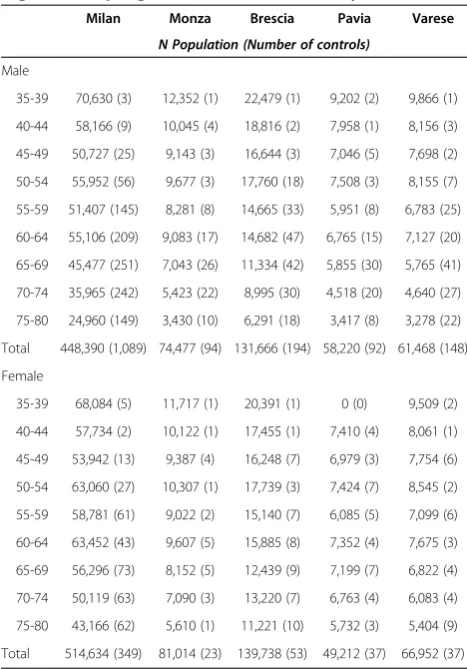
The EAGLE Study is a population-based case–control study of lung cancer in a Northern Italian population. Details of the study design have been previously de-scribed [10]. Briefly, during 34 months of observation between 2002–2005, 2,100 pathologically-confirmed cases of primary lung cancer were identified from 13 hospitals in the Lombardy region. A frequency-matched random sample of 2,120 controls was drawn from the Lombardy census using 90 strata defined by combina-tions of residence, age, and gender. Our analyses were based on the 1,943 cases (92.5%) and 2,116 controls (99.8%) who completed the study interview, and we as-sumed that the completion of an interview was non-informative for the risk association analyses. Table 1 shows the study’s sampling strata, the size of the control population, and the size of the control sample in each stratum. Approximate sampling fractions, the proba-bility of a control subject’s selection, are equal to the
control sample size divided by its population size.Lexpit analyses use the sampling information to estimate the association of selected exposures and the 3-year (rounded from 34 months) absolute risk of lung cancer. Since only a small percentage of cases and controls did not complete a study interview, population counts were derived from the interviewed sample without adjust-ment for interview completion.
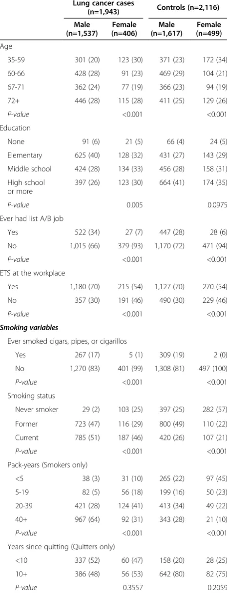
Table 2 summarizes information on demographics, smoking history, and environmental smoking exposure in the cases and controls of the study sample, after ex-cluding 157 cases and 4 controls without a complete baseline questionnaire. Men had greater smoking expos-ure than women overall, and in cases and controls separ-ately. While 98% of male cases and 75% of male controls were current or former smokers, 75% of female cases and 43% of female controls had ever smoked. Compared to women of the same case status, men were more likely to have held a high-risk job [14], been exposed to to-bacco smoke in the workplace, or to have smoked cigars, pipes, or cigarillos (Table 2).
Table 1 Projected control population by gender, age, and regional sampling strata in the EAGLE Study
Milan Monza Brescia Pavia Varese
N Population (Number of controls)
Male
35-39 70,630 (3) 12,352 (1) 22,479 (1) 9,202 (2) 9,866 (1)
40-44 58,166 (9) 10,045 (4) 18,816 (2) 7,958 (1) 8,156 (3)
45-49 50,727 (25) 9,143 (3) 16,644 (3) 7,046 (5) 7,698 (2)
50-54 55,952 (56) 9,677 (3) 17,760 (18) 7,508 (3) 8,155 (7)
55-59 51,407 (145) 8,281 (8) 14,665 (33) 5,951 (8) 6,783 (25)
60-64 55,106 (209) 9,083 (17) 14,682 (47) 6,765 (15) 7,127 (20)
65-69 45,477 (251) 7,043 (26) 11,334 (42) 5,855 (30) 5,765 (41)
70-74 35,965 (242) 5,423 (22) 8,995 (30) 4,518 (20) 4,640 (27)
75-80 24,960 (149) 3,430 (10) 6,291 (18) 3,417 (8) 3,278 (22)
Total 448,390 (1,089) 74,477 (94) 131,666 (194) 58,220 (92) 61,468 (148)
Female
35-39 68,084 (5) 11,717 (1) 20,391 (1) 0 (0) 9,509 (2)
40-44 57,734 (2) 10,122 (1) 17,455 (1) 7,410 (4) 8,061 (1)
45-49 53,942 (13) 9,387 (4) 16,248 (7) 6,979 (3) 7,754 (6)
50-54 63,060 (27) 10,307 (1) 17,739 (3) 7,424 (7) 8,545 (2)
55-59 58,781 (61) 9,022 (2) 15,140 (7) 6,085 (5) 7,099 (6)
60-64 63,452 (43) 9,607 (5) 15,885 (8) 7,352 (4) 7,675 (3)
65-69 56,296 (73) 8,152 (5) 12,439 (9) 7,199 (7) 6,822 (4)
70-74 50,119 (63) 7,090 (3) 13,220 (7) 6,763 (4) 6,083 (4)
75-80 43,166 (62) 5,610 (1) 11,221 (10) 5,732 (3) 5,404 (9)
Lexpitmodel Description
Thelexpitmodel relates risk factorsxandzto the abso-lute risk (also called cumulative risk of disease or the probability of disease) over a fixed time interval. Here, both x and z can include multiple categorical or con-tinuous variables. Denoting the absolute risk of disease within a fixed timeτ given xand z asR(x, z), the lexpit model of cumulative risk is
R xð ;zÞ ¼β0xþ expit γ0þγ 0
z
ð1Þ
a sum of additive β'x and multiplicative expit(γ0+γ'z) components, where expit(u) =esp(u)/(1 + exp(u)) is the inverse-logit (expit) function, which converts the log-odds uto the risk scale. An incidence rate can also be derived by dividing the cumulative riskR(x,z)by the length of the risk periodτ,⋅R(x,z)/τ, under the assumption of constant risk over the risk period. For case–control study designs, the risk period lengthτis typically equal to the duration of case ascertainment. When the additive terms oflexpitare set to zero, the model reduces to a strictly multiplicative logistic model; when the multiplicative terms are set to zero, the model reduces to a strictly additive binomial linear model.
The “additive” and “multiplicative” descriptions of the lexpitmodel coefficients refer to the effects of thexand zvariables on the baseline risk, or the cumulative risk of disease in unexposed individuals, denoted as R0=expit (γ0).According to (1), the risk in a person with x=x1 ex-posure isβ'x1greater than a person with x=x1-1; thus, each β coefficient is a risk difference associated with a unit increase in the corresponding xfactor, after adjust-ing for all remainadjust-ingxandzfactors.
In Equation (1), the risk in a person with z=z1 is a multiplicative factor of the baseline risk approximately equal to≈exp(γ'z1). The exponentiated value of each γ coefficient estimates the residual odds ratio associated with a unit increase in the correspondingzvariable, after adjustment for the risk due to x exposures and the Table 2 Descriptive characteristics by gender for the
EAGLE study
Lung cancer cases
(n=1,943) Controls (n=2,116)
Male (n=1,537)
Female (n=406)
Male (n=1,617)
Female (n=499)
Age
35-59 301 (20) 123 (30) 371 (23) 172 (34)
60-66 428 (28) 91 (23) 469 (29) 104 (21)
67-71 362 (24) 77 (19) 366 (23) 94 (19)
72+ 446 (28) 115 (28) 411 (25) 129 (26)
P-value <0.001 <0.001
Education
None 91 (6) 21 (5) 66 (4) 24 (5)
Elementary 625 (40) 128 (32) 431 (27) 143 (29)
Middle school 424 (28) 134 (33) 456 (28) 158 (31)
High school or more
397 (26) 123 (30) 664 (41) 174 (35)
P-value 0.005 0.0975
Ever had list A/B job
Yes 522 (34) 27 (7) 447 (28) 28 (6)
No 1,015 (66) 379 (93) 1,170 (72) 471 (94)
P-value <0.001 <0.001
ETS at the workplace
Yes 1,180 (70) 215 (54) 1,127 (70) 270 (54)
No 357 (30) 191 (46) 490 (30) 229 (46)
P-value <0.001 <0.001
Smoking variables
Ever smoked cigars, pipes, or cigarillos
Yes 267 (17) 5 (1) 309 (19) 2 (0)
No 1,270 (83) 401 (99) 1,308 (81) 497 (100)
P-value <0.001 <0.001
Smoking status
Never smoker 29 (2) 103 (25) 397 (25) 282 (57)
Former 723 (47) 116 (29) 800 (49) 110 (22)
Current 785 (51) 187 (46) 420 (26) 107 (21)
P-value <0.001 <0.001
Pack-years (Smokers only)
<5 38 (3) 31 (10) 265 (22) 97 (45)
5-19 82 (5) 56 (18) 199 (16) 50 (23)
20-39 421 (28) 124 (41) 413 (34) 49 (22)
40+ 967 (64) 92 (31) 343 (28) 21 (10)
P-value <0.001 <0.001
Years since quitting (Quitters only)
<10 337 (52) 60 (47) 158 (20) 28 (25)
10+ 386 (48) 56 (53) 642 (80) 82 (75)
P-value 0.3557 0.2059
Table 2 Descriptive characteristics by gender for the EAGLE study(Continued)
Avg. percent inhaled (Smokers only)
25 1 (0) 5 (2) 3 (0) 1 (0)
50 62 (4) 17 (6) 36 (3) 11 (5)
75 449 (30) 113 (37) 295 (24) 53 (24)
100 995 (66) 168 (55) 886 (73) 152 (70)
P-value <0.001 0.3905
ETS = Environmental tobacco smoke.
effects of remainingz. In logistic regression, coefficients are the adjusted log-odds ratios of odds having the form R(x,z)/(1−R(x,z)). Inlexpit regression, the log-odds ra-tios represented by the coefficientsγ involve odds of the form (R(x,x)−β'x)/(1−R(x,z), where R(x,z)−β'x is the risk that remains after subtracting the risk due to x exposures. Hence, we refer to the exponentiated coeffi-cients γ of the lexpit model as “residual odds ratios”. These residual odds ratios are directly comparable to the odds ratio associations in a logistic regression model ofz exposures fit to the subgroup of individuals without ex-posure to thexvariables, i.e., with x = 0.
The baseline risk parameterγ0is included in the expit for mathematical convenience, as no constraints are re-quired to ensure that R0=expit(γ0) is within the feasible 0–1 probability range.
Example 1: Interpretation of lexpit model coefficients
To illustrate the interpretation of the coefficients of the lexpit model, suppose we perform alexpit regression in the EAGLE Study to determine the risk difference in the 3-year risk of lung cancer associated with gender, con-trolling for the effect of smoking duration. The lexpit model in our example is
R xð 1;z1Þ ¼βx1þ expit γ0þγz1
ð2Þ
with univariate x1 for gender (1 = female, 0 = male) and univariate multiplicative term z1= Years Smoked, a con-tinuous variable. Under model (2), the 3-year risk differ-ence between a woman and a man with equal years smoked isR(1,z1)−(0,z1) =βThus,βis the difference in lung cancer risk between women and men, adjusted for smoking.
Next we consider the independent effect of a 30-year smoking duration. Under model (2), the residual log-odds is lgit(R(3, 30)) =γ0+ 30γ for a man and logit(R (1, 30)−β) =γ0+ 30γfor a woman who have smoked for 30 years. For each, the difference in the residual log-odds compared to a never smoker (the log-log-odds ratio) is 30γ. Thus, γ represents increase in the odds of lung cancer associated with an additional year’s duration of smoking, adjusted for gender.
Estimation
Application of lexpit regression to population-based case–control data can generate absolute risk and risk difference estimates when an unbiased representation of the underlying population is available. As with expansion estimators in survey estimation [15], weighing each ob-servation by its inverse sampling fraction, roughly, yields an estimate of the number of individuals representative of the “study base” [16]. To accommodate stratified sam-pling, we suppose the study base consists ofJstrata. Letij
index theith individual within the jth stratum. The data vector for this individual is {yij,xij,zij,wij}, where yij indi-cates case status,xijare additive risk factors,zijare
multi-plicative risk factors, andwijis the sampling weight. For a population-based case–control study with complete case ascertainment and random sampling of controls within strata, the sample weights equal 1 for all cases and the ra-tio of the populara-tion size Nj to the number of sampled controlsnj(Nj/nj) for controls in stratumj. The use of in-verse probabilities as sampling weights allows our meth-odology to accommodate more complex case–control designs (frequency matching, individual matching, etc.).
We use constrained maximum likelihood methods to obtain estimates for the parameters of the lexpitmodel, maximizing the pseudo-log-likelihood
l β;γ0;γ
¼ΣjΣiwij
yijlogit R xij;zij
þ log 1−R xij;zij
h i
ð3Þ
If all sampling weightswijwere equal to 1, as in a co-hort design, Equation (3) would be the exact log-likelihood of a sample of Bernoulli random variablesyij, with expected event probabilities E[yij= 1] =R(xij,zij). The pseudo-likelihood approach extends the method proposed by Benichou and Wacholder [17] with add-itional constraints in the maximization to ensure that the estimated risks for all observed risk types are within the [0, 1] range. Estimates for Θ= (β,γ0,γ) are therefore the solutions to the following constrained optimization problem,
^
Θ¼ arg maxΘflð ÞΘ gandΘ∈F
where argmaxx{f(x)} is the value of x where f(x) achieves its maximum value andF defines the feasible region for the parameter space,
F¼0≤β0xþ expitγ0þγ0z≤1 forall xð ;zÞ∈ðX;ZÞ
The quantities X and Z refer to the complete set of risk factors in the study sample. The feasible region is constructed from the joint distribution of (X, Z), creat-ing a separate constraint for each unique combination of observedx andzfactors. The feasible region guarantees that the risk estimate for each observed exposure type is a population probability.
estimation of standard errors of estimates. We therefore use influence-based methods, a common approach for linearized variance estimation of survey statistics [18], to derive variances for thelexpitmodel’s risk estimates. In the Additional file 1 we summarize the optimization algorithm and the influence approach for obtaining variance estimates for thelexpitmodel parameters.
Example 2: Lexpit model estimation for case–control data
To illustrate the basic estimation concept, consider alexpit model with a single additive effect for gender xij (1 = fe-male, 0 = male),R(xij, 0) =βxij= expit(γ0). Table 1 indicates that 1,617 male controls were sampled from a population of 774,221; 499 female controls from a population of 851,550. Treating gender as the only stratification variable, the sampling weight for male controls was 774,221/ 1,61≈479 and for female controls was 851,550/499≈1,706. Given 1,537 total male cases and 406 total female cases of lung cancer during the 3-year ascertainment period, the weighted estimate for 3-year lung cancer risk in men is
expit γ^0 ¼
1;537 1;537þ7741;617;2211;617
¼ 1;537
1;537þ4;221≈2:0=1;000
and for women
expit γ^0 þ^β
406
406þ851499;550499¼
406 406þ851;550
≈0:5=1;000
A risk difference estimate of ^β¼−1:5=1;000 repre-sents 0.15% lower risk for women than men This ex-ample conceptualizes how the sampling probabilities of a case–control study, when available, can be utilized to obtain population risk estimates.
Choice of additive and multiplicative effects
The flexibility oflexpitregression in allowing estimation of the effect of an exposure as additive, multiplicative, or (in some cases) both, can create uncertainty about an exposure’s true mode of effect. Although thetrue mode of effect can never be known, we provide three practical strategies to explore the functional form of a given risk-exposure relationship: a risk-risk-exposure scatter plot that gives a graphical depiction between crude risk and a continuous exposure, a testing method based on the comparison of effects in a lexpit model with both addi-tive and multiplicaaddi-tive effects of an exposure, and a measure of goodness-of-fit. Details of each approach are provided in the Additional file 1.
Results
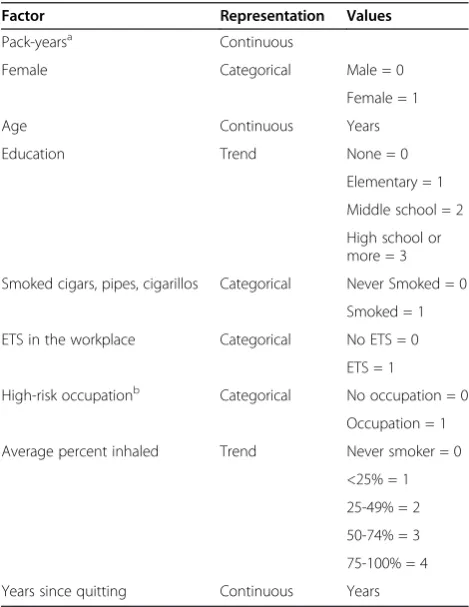
Lexpit regression was performed to assess the absolute risk differences associated with gender and smoking in the Northern Italian population represented by EAGLE partic-ipants. Our main interest was in a model that could esti-mate additive effects for gender, pack-years, and their interaction, considering multiplicative effects for all remai-ning covariates. A description of the included variables and their codings are described in Table 3. Thelexpit ana-lysis was conducted in the R language, version 2.15 [19], using our open-source package blm [20] (for usage exam-ples see Additional file 2 and Additional file 3).
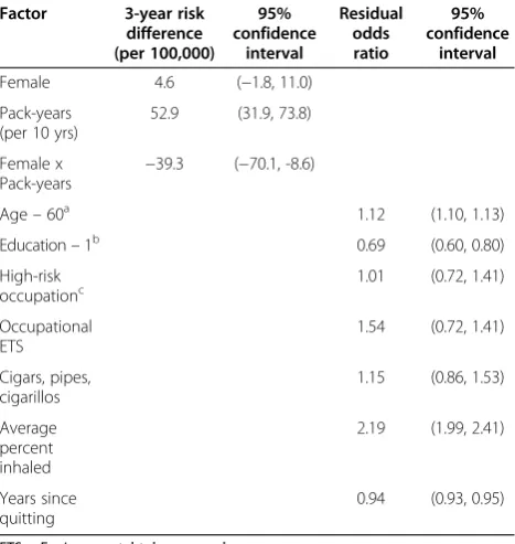
Estimates for the additive effects of gender showed a 4.6 per 100,000 persons higher 3-year lung cancer risk for women than men among never smokers, adjusting for other demographic variables (Table 4). The risk difference effect can also be expressed as a rate by dividing by the duration of risk, e.g. a 4.6 per 100,000 34-month risk cor-responds to an average risk rate of 13 per 100,000 person-years. We estimate that every 10 additional pack-years smoked increases the 3-year lung cancer risk in male smokers by 52.9 per 100,000 persons but by only 13.6 per 100,000 persons among women, showing a strong
female-Table 3 Representation of variables included in regression analyses of the EAGLE study
Factor Representation Values
Pack-yearsa Continuous
Female Categorical Male = 0
Female = 1
Age Continuous Years
Education Trend None = 0
Elementary = 1
Middle school = 2
High school or more = 3
Smoked cigars, pipes, cigarillos Categorical Never Smoked = 0
Smoked = 1
ETS in the workplace Categorical No ETS = 0
ETS = 1
High-risk occupationb Categorical No occupation = 0
Occupation = 1
Average percent inhaled Trend Never smoker = 0
<25% = 1
25-49% = 2
50-74% = 3
75-100% = 4
Years since quitting Continuous Years
ETS = Environmental tobacco smoke.
a
Average packs of cigarettes smoked per day x years smoked.
b
pack-year interaction (RD=−39.3 per 100,000 persons per 10 pack-years smoked, 95% CI=−70.1 to −8.6). After ac-counting for the risk effects of gender and pack-years, the residual odds ratio effects of the lexpitmodel found that greater age, occupational ETS exposure, and inhalation depth further increased lung cancer risk estimates, while higher education and greater years since quitting de-creased risk estimates.
As one assessment of the improvement of the fit of the model with the use of multiplicative effects we com-pared the weighted Hosmer-Lemeshow goodness-of-fit statistic (Additional file 1: Section S3) among the lexpit model, a strictly additive blm model, and a strictly mul-tiplicative logistic model of the same variables. The chi-squared statistic in the blm model was 20.8, the weighted logistic model 18.2, and 15.9 with the lexpit model, indicating an improvement in fit with the use of the additive-multiplicative form we used.
Discussion
We have presentedlexpitregression methods to estimate adjusted absolute risk differences with population-based case–control data. By shifting the focus from estimates of relative risk to absolute risk,lexpitregression gives epide-miologists a direct and reliable way to assess the public health significance of an exposure’s effect. Moreover,lexpit regression provides a flexible framework for handling po-tential confounders, as variables with additive or multi-plicative effects can be accommodated. When there is
uncertainty about a variable’s mode of effect, we outlined approaches to assess the reasonableness of each effect type. Our open-source R package blm allows the new methods to be implemented with the ease of standard lo-gistic regression.
Lexpitregression is the absolute risk analog to additive-multiplicative models for hazard rates, such as the Cox-Aalen model [21], which have become increasingly popular in the survival literature [22]. Each class of models share the strength of greater flexibility in the study and representation of the joint effects of risk factors on the hazard rate, in the case of the Cox-Aalen model, and the absolute risk of disease, in the case of the lexpitmodel. The extension of additive-multiplicative models to abso-lute risk estimation from a variety of study designs is sig-nificant because of the importance of individualized risk assessment to public health. To our knowledge, thelexpit model is the first additive-multiplicative regression model of risk that appropriately ensures risk estimates are within the probability scale. Although alternative additive-multiplicative models of risk could be developed by con-sidering other functions for the multiplicative component (e.g. exp), we have focused on theexpitfunction because of its mathematical advantages. Because of the expit func-tion, the lexpitmodel will require fewer constraints than alternative additive-multiplicative models to produce feas-ible estimates in the 0–1 probability range.
None of more than 20 published observational studies that have examined male–female differences in lung cancer etiology have quantified the independent effect of gender on the absolute risk of smoking- and non-smoking-associated lung cancer [23-26]. Usinglexpitregression, we were able to address this important public health question. Our findings add to the De Matteiset al.logistic regression of the EAGLE case–control study [11] in two important ways. First, we confirmed that gender differences in the confounder-adjusted effect of pack-years are found on the additive risk scale. Secondly, we found suggestive evidence that women’s risk of lung cancer risk is higher than men’s in never smokers but is lower than men’s in smokers. Con-ventional unconditional logistic regression, which does not provide estimates of absolute risk, would not identify these findings, especially given that gender was used as a match-ing variable in selectmatch-ing controls. Thus, our novel methods provide further insight about male-and-female differences in lung cancer risk from previously analyzed data that has direct public health implications.
In their commentary on the De Matteis et al. study, Alberg and colleagues pointed to a need to further delin-eate the clinical significance of gender differences in lung cancer etiology [12]. Our re-analysis of the EAGLE Study clarifies the clinical relevance of gender effects for lung cancer risk in an Italian population by providing es-timates of the excess lung cancer risk associated with Table 4Lexpitregression analysis of the EAGLE Study
Factor 3-year risk difference (per 100,000)
95% confidence
interval
Residual odds ratio
95% confidence
interval
Female 4.6 (−1.8, 11.0)
Pack-years (per 10 yrs)
52.9 (31.9, 73.8)
Female x Pack-years
−39.3 (−70.1, -8.6)
Age–60a 1.12 (1.10, 1.13)
Education–1b 0.69 (0.60, 0.80)
High-risk
occupationc 1.01 (0.72, 1.41)
Occupational ETS
1.54 (0.72, 1.41)
Cigars, pipes, cigarillos
1.15 (0.86, 1.53)
Average percent inhaled
2.19 (1.99, 2.41)
Years since quitting
0.94 (0.93, 0.95)
ETS = Environmental tobacco smoke.
a
Centered at 60 years.
b
Centered at 1, corresponding to elementary school.
c
gender. The small excess risk in women never smokers suggests that some gender-related etiological factor(s) for non-smoking-related lung cancer remains to be iden-tified. A public health implication for the gender differ-ences we found among smokers concerns selection criteria for computed tomographic lung cancer screen-ing. Current guidelines recommend screening for indi-viduals between ages 55 and 75 years with a minimum of 30 pack-years smoked [27]. However, in an Italian population, we estimate that the excess lung cancer risk for a male 30 pack-year smoker is more than 1,100 per 100,000 greater than an otherwise similar female 30 pack-year smoker. Thus, in keeping with the “equal management for equal risk” principle [28], gender-based risk criteria for lung cancer screening selection may be warranted in some populations.
The implications of the EAGLElexpitanalysis for com-puted tomographic screening guidelines exemplifies the importance of the choice of measure of association used in an etiological analysis for understanding the public health significance of a risk factor’s effect. Risk differences meas-ure a risk factor’s effect in terms of the number of excess attributable cases in a well-defined population, an explicit measure of the public health significance of an effect, which can be compared across exposures and across dis-eases. Our study provides an important example of this comparative use of risk differences with respect to gender effects in smoking- and non-smoking-associated lung can-cer. Some research has suggested a higher risk of lung cancer among women never smokers [29]. We further elu-cidated this difference throughlexpit analysis by showing that the excess risk in women never smokers was approxi-mately equal to the excess risk with 1 additional pack-year smoked in men as compared to women. As the develop-ment of public health interventions and clinical recom-mendations become increasingly guided by individual risk assessment, there will be a growing need for methods like lexpitregression that can facilitate the estimation of abso-lute risk differences from observational data.
Lexpitregression resolves several limitations of alterna-tive strategies for estimating risk differences from case– control studies. Using non-additive models of risk, such as the logistic model, to estimate a marginal risk difference [30,31] gives average in the study population, not equiva-lent to a risk difference effect estimated here. The applica-tion of the lexpit model to case–control data extends previously proposed methods for absolute risk methods requiring prospective cohorts or disease registries [32]. Further, lexpit regression advances current methods for assessing additive interactions in case–control studies. It is well known that multiplicative interactions sometimes dis-appear when modeled on the additive scale [4-6,33] and vice versa, highlighting the dependence of statistical inter-actions on the choice of a model’s scale. The removal of
interactions leads to more parsimonious models whose risk associations have a clearer interpretation. The flexible additive-multiplicative form of the lexpitcan help epide-miologists reduce multiplicative and additive statistical in-teractions, making it easier to interpret risk effects. While departure from additivity can be detected on the relative risk scale using the relative excess risk due to interaction, this metric is limited because it can only detect the direc-tion of departure from additivity but not the magnitude of the effect [34,35].
Whilelexpitregression makes the important advance of allowing case–control studies to make inferences about absolute risk and risk differences of exposures, there are several challenges to its application to case– control data. First, the period of risk for the cumulative risk estimates of the lexpitmodel is determined by the period of case ascertainment, which may generally pro-hibit long-term risk estimates. As with other common probability models of case–control data, the lexpit model assumes the population risk of disease is fixed during the period cases and controls are sampled. The population validity oflexpitregression also requires ac-curate sampling weights, which may be difficult to ob-tain for studies using a so-called “secondary base” [36], as with hospital or registry controls, for the selection of controls. Further investigation of the availability and ac-curacy of sampling information in case–control studies is needed to clarify the practical limitations of using sampling data for absolute risk estimation.
Conclusions
Additive and multiplicative models concern “two quite different aspects of the association between risk factor and disease” [1], p. 58. Epidemiologists have been urged to consider both perspectives in risk association studies, especially in the assessment of effect modification [26], yet technical challenges have long made multiplicative models more convenient to use. In this paper, we have presented methods and software [27] to allow analyses of population-based case–control studies to incorporate these complementary perspectives into a single model vialexpitregression. Further applications and extensions of additive risk modeling with case–control data will help to improve our understanding of the joint effects of exposures on disease risk.
Additional files
Additional file 1:Supplementary technical appendix.
Additional file 2:R script file showing examples of lexpit modeling and supporting functions using the R blm package.
Additional file 3:Simulated population-based case–control dataset
modeled after the EAGLE study design.The examples presented in
Abbreviations
EAGLE:Environment and genetics in lung cancer etiology; Lexpit: Linear-expit.
Competing interests
The authors have no competing interests to declare.
Authors’contributions
SAK designed and conducted the study analyses and wrote the first draft of the manuscript. SW, NEC, and MTL conceived of the design of the study sample and the coordination of data collection. SW, HAK, SDM, DC, AWB, and RV provided input on the statistical analyses and the interpretation of the results. All authors contributed to the writing of the manuscript and read and approved the final manuscript.
Acknowledgement
This work was supported by the Intramural Research Program of the National Institutes of Health, National Cancer Institute, Division of Cancer Epidemiology and Genetics. Dr. Varadhan is a Brookdale Leadership in Aging Fellow at the Johns Hopkins University School of Medicine.
Author details
1Economics, Sociology, and Statistics Department, RAND Corporation, Santa
Monica, CA, USA.2Unit of Epidemiology, Department of Preventive Medicine,
Fondazione IRCCS Ca’Granda - Ospedale Maggiore Policlinico, Milan, Italy.
3
Division of Cancer Epidemiology and Genetics, National Cancer Institute, National Institutes of Health, Bethesda, MD, USA.4Division of Geriatric
Medicine and Gerontology, Department of Medicine, Johns Hopkins University School of Medicine, Baltimore, MD, USA.5Molecular Genetics
Program, Center for Health Sciences, SRI International, Menlo Park, CA, USA.
Received: 25 July 2013 Accepted: 7 November 2013 Published: 19 November 2013
References
1. Breslow NE, Day NE:Statistical Methods in Cancer Research, Vol. I. The Design and Analysis of Case–control Studies, IARC Scientific Publication No. 32. New York, NY: Oxford University Press; 1980.
2. Greenland S:Interpretation and choice of effect measures in epidemiologic analyses.Am J Epidemiol1987,125(5):761–768. 3. Sackett DL, Deeks JJ, Altman DG:Down with odds ratios!Evid Based Med
1996,1:164–166.
4. Skrondal A:Interaction as departure from additivity in case–control studies: a cautionary note.Am J Epidemiol2003,158:251–258. 5. Rothman KJ:Causes.Am J Epidemiol1976,104:587–593.
6. Knol MJ, VanderWeele TJ:Recommendations for presenting analyses of effect modification and interaction.Int J Epidemiol2012,41:514–520. 7. Wacholder S:The case–control study as data missing by design:
estimating risk differences.Epidemiol1996,7(2):144–150.
8. Wacholder S:Binomial regression in GLIM: estimating risk ratios and risk differences.Am J Epidemiol1986,123:174–184.
9. Spiegelman D, Hertzmark E:Easy SAS calculations for risk or prevalence ratios and differences.Am J Epidemiol2005,162(3):199–200.
10. Landi MT, Consonni D, Rotunno M, Bergen AW, Goldstein AM, Lubin JH, Goldin L, Alavanja M, Morgan G, Subar AF, Linnoila I, Previdi F, Corno M, Rubagotti M, Marinelli B, Albetti B, Colombi A, Tucker M, Wacholder S, Pesatori AC, Caporaso NE, Bertazzi PA:Environment and genetics in lung cancer etiology (EAGLE) study: an integrative population-based case–control study of lung cancer.BMC Public Health2008,8:203. 11. De Matteis S, Consonni D, Pesatori AC, Bergen AW, Bertazzi PA, Caporaso NE,
Lubin JH, Wacholder SW, Landi MT:Are women who smoke at higher risk for lung cancer than men who smoke?Am J Epidemiol2013,177(7):601–612. 12. Alberg AJ, Wallace K, Silvestri GA, Brock MV:Invited commentary: the
etiology of lung cancer in men compared with women.Am J Epidemiol 2013,177(7):613–616.
13. Kovalchik SA, Varadhan R, Fetterman B, Poitras NE, Wacholder S, Katki HA: A general binomial regression model to estimate standardized risk differences from binary response data.Stat Med2013,32:808–821. 14. Consonni D, De Matteis S, Lubin JH, Wacholder S, Tucker M, Pesatori AC,
Caporaso NE, Bertazzi PA, Landi MT:Lung cancer and occupation in a
population-based case–control study.Am J Epidemiol2010, 171(3):323–333.
15. Horvitz DG, Thompson DJ:A generalization of sampling without replacement from a finite universe.J Am Stat Assoc1952,47:663–685. 16. Wacholder S, Silverman DT, McLaughlin JK, Mandel JS:Selection of controls
in case–control studies: 2. Types of controls.Am J Epidemiol1992, 135(9):1029–1041.
17. Benichou J, Wacholder S:A comparison of 3 approaches to estimate exposure-specific incidence rates from population-based case–control data.Stat Med1994,13:651–661.
18. Graubard BI, Fears TR:Standard errors for attributable risk for simple and complex sample designs.Biometrics2005,61(3):847–855.
19. R Development Core Team:R: A Language and Environment for Statistical Computing.Vienna, Austria: R Foundation for Statistical Computing; 2012. 20. Kovalchik SA, Varadhan R:Fitting additive binomial regression models
with the R package blm.J Stat Softw2013,54(1):1–18.
21. Martinussen T, Scheike TH:A flexible additive-multiplicative hazard model. Biometrika2002,89(2):283–298.
22. Cortese G, Scheike TH, Martinussen T:Felxible survival regression modelling.Stat Methods Med Res2010,19(1):5–28.
23. Blot WJ, McLaughlin JK:Are women more susceptible to lung cancer? J Natl Cancer Inst2004,96(11):812–813.
24. Khuder SA:Effect of cigarette smoking on major histological types of lung cancer: a meta-analysis.Lung Cancer2001,31(2–3):139–148. 25. Bain C, Feskanich D, Speizer FE, Thun M, Hertzmark E, Rosner BA, Colditz GA:
Lung cancer rates in men and women with comparable histories of smoking.J Natl Cancer Inst2004,96(11):826–834.
26. Gandini S, Botteri E, Iodice S, Boniol M, Lowenfels AB, Maisonneuve P, Boyle P:Tobacco smoking and cancer: a meta-analysis.Int J Cancer2008, 122(1):155–164.
27. Boiselle PM:Computed tomography screening for lung cancer. JAMA2013,309:1163–1170.
28. Katki HA, Schiffman M, Castle PE, Fetterman B, Poitras NE, Lorey T, Cheung LC, Raine-Bennett T, Gage JC, Kinney WK:Five-year risks of CIN 2+ and CIN 3+ among women with HPV-positive and HPV-negative LSIL pap results.J Low Genit Tract Dis2013,17:S43–S49.
29. Wakelee H, Chang E, Gomez S, Keegan T, Feskanich D, Clarke C, Holmberg L, Yong L, Kolonel L, Gould M,et al:Lung cancer incidence in never smokers. J Clin Oncol2007,25(5):472–478.
30. Greenland S, Holland P:Estimating standardized risk differences from odds ratios.Biometrics1991,47(1):319–322.
31. Greenland S:Model-based estimation of relative risks and other epidemiologic measures in studies of common outcomes and in case–control studies.Am J Epidemiol2004,160(4):301–305.
32. Benichou J, Gail MH:Methods of inference for estimates of absolute risk derived from population-based case–control studies.Biometrics1995, 51(1):182–194.
33. Marschner IC, Gillett AC, O’Connell RL:Stratified additive Poisson models: computational methods and applications in clinical epidemiology. Comput Stat Data Anal2012,56(5):1115–1130.
34. Knol MJ, van der Tweel I, Grobbee DE, Numans ME, Geerlings MI: Estimating interaction on an additive scale between continuous determinants in a logistic regression model.Int J Epidemiol2007, 36:1111–1118.
35. Richardson DB, Kaufman JS:Estimation of the relative excess risk due to interaction and associated confidence bounds.Am J Epidemiol2009, 169(6):756–760.
36. Wacholder S, McLaughlin JK, Silverman DT:Selection of controls in case–control studies: 1. Principles.Am J Epidemiol1992,135(9):1019–1028. doi:10.1186/1471-2288-13-143