Sensorless control of brushless permanent magnet motors

(1)

SENSORLESS CONTROL OF BRUSHLESS

PERMANENT MAGNET MOTORS

CHAWANAKORN MANTALA

A thesis submitted in partial fulfilment of the

requirements of the University of Bolton

for the degree of Doctor of Philosophy

This research programme was carried out

in collaboration with

South Westphalia University of Applied Sciences

Department of Electrical Energy Technology

Soest, Germany

(2)

Declaration

I declare that I have developed and written the enclosed thesis entitled, “ Sensorless Control of Brushless Permanent Magnet Motors,” by myself and have not used sources or means without declaration in the text. Any thoughts or quotations which are inferred from these sources are clearly marked.

This thesis was not submitted in the same or in a substantially similar version, not even portion of the work, to any authority to achieve any other qualification.

December 2013,

(3)

Abstract

In this thesis, a sensorless control method of permanent magnet synchronous machines (PMSMs), whose machine neutral points are accessible, for all speeds and at standstill is proposed, researched and developed. The sensorless method is called Direct Flux Control (DFC). The different voltages between a machine neutral point and an artificial neutral point are required for the DFC method. These voltages are used to extract flux linkage signals as voltage signals, which are necessary to approximate electrical rotor positions by manipulating the flux linkage signals. The

DFC method is a continuous exciting method and based on an asymmetry characteristic and machine saliencies.

The DFC method is validated by implementing on both software and hardware implementation. A cooperative simulation with Simplorer for the driving circuit and programming the DFC and Maxwell for doing finite element analysis with the machine design is selected as the software simulation environment. The machine model and the DFC method are validated and implemented. Moreover, the influences of different machine structures are also investigated in order to improve the quality of the measured voltages.

The hardware implementation has been employed on two test benches, i.e. for small machines and for big machines. Both test benches use a TriCore PXROS microcontroller platform to implement the DFC method. There are several PMSMs, both salient poles and non-salient poles, which are used to validate the DFC method. The flux linkage signals are also analyzed. The approximation of the flux linkage signal is derived and proposed. A technique to remove the uncertainty of the calculated electrical rotor position based on the inductance characteristics has been found and implemented. The electrical rotor position estimation method has been developed based on the found flux linkage signal approximation function and analyzed by comparing with other calculation techniques.

Moreover, the calculated electrical rotor position is taken into account to either assure

(4)

presented and executed by using the assured calculated electrical rotor position to perform the DFC capability.

This thesis has been done in the Electric Machines, Drives and Power Electronics Laboratory, South Westphalia University of Applied Sciences, Soest, Germany.

Keywords: Direct Flux Control (DFC), Permanent Magnet Synchronous Machine

(5)

Acknowledgement

First of all, I wish to thank and place on record my immense gratitude to my supervisor Prof. Dr.-Ing. Peter Thiemann for his continuous support, sponsor, guidance and supervision, Mr. Karl-Heinz Weber and Mr. Tobias Müller for kind assistance and in general to everyone who works in the Electric Machines, Drives and Power Electronics Laboratory, South Westphalia University of Applied Sciences, Soest, Germany. In addition, I would like to thank Dr. Rolf Strothmann, who patented this method and supported on this research including Dr. Willi Theiß, HighTec

EDV-Systeme GmbH, Saarbruecken, Germany.

Furthermore, I would like to record my thankfulness to Dr. Erping Zhou from the University of Bolton (UK) who participated her time to be the supervisor in this thesis.

Finally, my deepest thank also goes to my parents, Mrs. Sumitta and Mr. Manit Mantala, my brother, Mr. Kantapol Mantala , family , friends, especially Mr. Paramet Wirasanti, and everyone who encouraged me throughout while working on this thesis.

December 2013,

(6)

List of Figures

Fig. 1.1: FOC of Permanent Magnet Synchronous Machine ... 2

Fig. 2.1: Structure of ELO... 7

Fig. 2.2: Structure of EKF ... 7

Fig. 2.3: Structure of SMO ... 8

Fig. 2.4: Proposed sliding function ... 8

Fig. 2.5: Measurement sequences of phase U [12] ... 10

Fig. 2.6: INFORM time diagram [12] ... 10

Fig. 2.7: Carrier signal injection ... 11

Fig. 2.8: Zero sequence voltage signal measuring scheme ... 12

Fig. 2.9: Current derivatives measuring scheme ... 12

Fig. 2.10: Line to neutral voltage measuring scheme ... 13

Fig. 3.1: Flux linkage extraction measuring scheme... 16

Fig. 3.2: Applied pulse pattern ... 17

Fig. 3.3: Machine equivalent circuit of each state ... 17

Fig. 3.4: Assumed flux linkage signals (u: red, v: blue, w: green) ... 20

Fig. 3.5: Calculated electrical rotor position ... 21

Fig. 3.6: Manipulated calculated electrical rotor position ... 22

Fig. 3.7: DFC electrical rotor position (αcal) ... 22

Fig. 3.8: PMSM1 ... 23

(11)

Fig. 3.10: PMSM3 ... 24

Fig. 3.11: Combination of software environments... 26

Fig. 3.12: 2D PMSM Model ... 26

Fig. 3.13: FEM model validation ... 27

Fig. 3.14: Applied constant input at PM = 20% ... 28

Fig. 3.15: Applied a constant speed to load machine at 35 rpm ... 29

Fig. 3.16: Connected PMSM1 with TriCore PXROS platform ... 31

Fig. 3.17: Test bench for small machines ... 31

Fig. 3.18: Step input at PM = 10% ... 31

Fig. 3.19: Applied step input experimental results ... 32

Fig. 3.20: Varied input pattern ... 33

Fig. 3.21: Applied varied input experimental results ... 34

Fig. 3.22: Test bench for big machines ... 35

Fig. 3.23: Varied input pattern ... 36

Fig. 3.24: Applied varied input experimental results ... 37

Fig. 3.25: PMSM3 flux linkage signals (u: red, v: blue, w: green) ... 38

Fig. 3.26: DFC Diagram ... 38

Fig. 4.1: DFC timing diagram ... 40

Fig. 4.2: Applied Disturbance on PMSM1... 42

Fig. 4.3: Applied Disturbance on PMSM2... 43

(12)

Fig. 4.5: Approximated flux linkage signal ... 45

Fig. 4.6: Flux relations in stationary frame ... 46

Fig. 4.7: Each modified PMSM electrical rotor position ... 47

Fig. 4.8: Calculated electrical rotor position errors... 48

Fig. 4.9: Each modified PMSM VNAN ... 48

Fig. 4.10: Each modified PMSM Tm ... 48

Fig. 5.1: Space vector diagram on TriCore PXROS platform ... 51

Fig. 5.2: PMSM stator diagram ... 55

Fig. 5.3: Flux linkage extraction measuring scheme... 57

Fig. 5.4: Four states of VN ... 58

Fig. 5.5: Four states of VNAN ... 59

Fig. 5.6: DFC timing diagram ... 63

Fig. 5.7: Calculated flux linkage signals (u: red, v: blue, w: green)... 67

Fig. 5.8: Time constant to measure VNAN of PMSM1 (VU : Ch1, VV : Ch2, VW : Ch3, IU : Ch4) ... 68

Fig. 5.10: Time constant to measure VNAN of PMSM2 (VU : Ch1, VV : Ch2, VW : Ch3, IU : Ch4) ... 69

Fig. 5.12: Flux linkage weakening and strengthening signals ... 72

Fig. 5.13: Flux linkage signals (u, v, w) ... 73

(13)

Fig. 5.15: ₁ correct position ... 75

Fig. 5.16: ₁ incorrect position... 76

Fig. 6.1: Calculated flux linkage signals (u: red, v: blue, w: green)... 78

Fig. 6.2: _{cal Ph}_, ... 79

Fig. 6.3: _{cal Pl}_, ... 80

Fig. 6.4: _{cal PF}_, ... 82

Fig. 6.5: 2D relation (  7) ... 82

Fig. 6.6: cal PF, (  21) ... 83

Fig. 6.7: 2D relation (  21) ... 83

Fig. 6.8: Position signals (PLU,raw : red, PLV,raw : blue, PLW,raw : green) ... 86

Fig. 6.9: Position signal without offsets (PLU : red, PLV : blue, PLW : green) ... 87

Fig. 6.10: _{cal PL}_, ... 88

Fig. 6.11: 2D relation of position signals ... 88

Fig. 6.12: Influence of offset through spectrum ratio of position signals ... 89

Fig. 6.13: Error of estimated rotor positon ... 90

Fig. 6.14: PMSM4 ... 91

Fig. 6.15: New test bench for big machines ... 92

Fig. 6.16: Incremental encoder signals in one mechanical round ... 93

Fig. 6.17: Coupled shaft motor ... 94

(14)

Fig. 6.19: Influence of Voffset through PMSM4 position signals ... 96

Fig. 6.20: u and PLU at 60 rpm ... 97

Fig. 6.21: v and PLV at 60 rpm ... 97

Fig. 6.22: w and PLW at 60 rpm ... 98

Fig. 6.23: Spectrum of at 60 rpm ... 99

Fig. 6.24: Spectrum of PLU at 60 rpm ... 99

Fig. 6.25: 2D relation of flux linkage signals at 60 rpm ... 100

Fig. 6.26: 2D relation of position signals at 60 rpm ... 100

Fig. 6.27: Phase shift between _{cal PF}_, and _{cal PL}_, ... 101

Fig. 6.28: _{cal PL}_, _{cal PF}_, ... 102

Fig. 6.29: Mechanical rotor position estimation _{R cal}_, ... 104

Fig. 6.30: _Rand cal PF, (PM = 25%) ... 105

Fig. 6.31: Rand cal PL, (PM = 25%) ... 105

Fig. 6.32: _{R cal PF}_, _, and _{R cal PL}_, _, (PM = 25%) ... 106

Fig. 6.33: err_{R cal PF}_, _, and err_{R cal PL}_, _, [Degree] (PM = 25%) ... 106

Fig. 6.34: LU of PMSM4 ... 108

Fig. 7.1: DFC Diagram ... 110

Fig. 7.2: DFC diagram with currents measurement ... 112

Fig. 7.3: Structure of current measurement ... 112

(15)

Fig. 7.5: Relation between PM and the resultant voltage vector... 115

Fig. 7.6: DFC input calculation ... 115

Fig. 7.7: Internal loop ... 115

Fig. 7.8: Experimental environment for current loop ... 117

Fig. 7.9: Iq step response ... 118

Fig. 7.10: Id step response ... 119

Fig. 7.11: Central loop ... 120

Fig. 7.12: Iq,s step input ... 120

Fig. 7.13: Iq,m and Id,mof Iq,s step input ... 121

Fig. 7.14: Id,s step input ... 121

Fig. 7.15: Iq,m and Id,mof Id,s step input ... 122

Fig. 7.16: Iq,s and Id,s step inputs... 122

Fig. 7.17: Iq,m and Id,mof Iq,s and Id,s step inputs ... 123

Fig. 7.18: Adding speed calculation to central loop... 124

Fig. 7.19: Iq,m and Id,m (Iq,s at 5 A) ... 124

Fig. 7.20: Calculated mechanical rotor speed (Nm) ... 125

Fig. 7.21: Closed loop speed sensorless control with DFC ... 127

Fig. 7.22: Required characteristics for closed loop control ... 127

Fig. 7.23: Zoomed _cal and Iq,m ... 128

Fig. 7.24: Flipping rotor direction closed loop speed control experimental results .. 129

(16)

Fig. 7.26: Zoomed stopped rotor closed loop speed control results... 130

Fig. 7.27: Applied TL at standstill (Ns=0 rpm) ... 131

Fig. 7.28: Applied TL while driving the machine (Ns=600 rpm) ... 132

Fig. 7.29: Spectrum of Iq,m at Nm 600 rpm ... 133

Fig. 8.1: Flux relations in stationary frame ... 139

(17)

List of Tables

Table 2.1: Categorization of machine saliencies based sensorless methods (refer to the numbers of references) ... 9

Table 4.1: PMSM structure analysis results ... 49

Table 10.1: Machine phase current (Irms) by normal connection ... r

(18)

List of Symbols

p Subscript stands for the phase U, V, W raw Subscript stands for raw information

s Subscript stands for strengthening signal

w Subscript stands for weakening signal

' Superscript stands for the first derivative by time

 Electrical rotor position [rad, °]

cal

 Calculated electrical rotor position [rad, °]

m

 Summation of calculated electrical rotor position and electrical correction angle [rad, °]

k

 Electrical correction angle [rad, °]

R

 Mechanical rotor position [rad, °]

,

R cal

 Estimated mechanical rotor position [rad, °]

,

cal m

 Calculated electrical rotor position by m method [rad, °]

( , )  Stationary frame

 Ratio between L_xand L_y



 Flux in  axis [Wb , Vs]



 Flux in  axis [Wb , Vs]

d

 Flux in d axis [Wb , Vs]

(19)

*

 Coupled flux linkage of other phases including the permanent rotor

flux [Wb , Vs]

p

 Resultant flux linkage of phase p [Wb , Vs]

r

 Rotor flux [Wb , Vs]

s

 Stator flux [Wb , Vs]

t

 Total flux [Wb , Vs]

 Time constant of RL circuit [s]

d

 Time constant in d axis [s]

q

 Time constant in q axis [s]

s

 Time constant for speed control [s]

 Sampling frequency [rad/s]



 Electrical frequency [rad/s]

R

 Mechanical frequency [rad/s]

( , )d q Synchronous frame

,

cal m

err Error of the calculated electrical rotor position by m method [rad, °]

d

I Current in d axis [A]

,

d m

I Measured current in d axis [A]

,

d s

I Desired current in d axis [A]

q

(20)

,

q m

I Measured current in q axis [A]

,

q s

I Desired current in q axis [A]

sum

I Summation of phase currents [A]

J Moment of inertia [kgm2]

k Multiplication factor of position signal by using phase inductance [ V1/2H-1]

C

K Gain of PI controller

p

L Machine phase inductance of phase p [H]

*p

L_ Combined form of machine phase inductance of phase p [H]

d

L Inductance in d axis [H]

ds

L Inductance in d axis while strengthening the magnetic field [H]

dw

L Inductance in d axis while weakening the magnetic field [H]

q

L Inductance in q axis [H]

x

L Summation of Ldand Lq [H]

y

L Difference between Ldand Lq [H]

s

N Desired mechanical speed [rpm, s-1]

m

N Calculated mechanical speed [rpm, s-1]

p

PL Position signal by using phase inductance of phase p [ V1/2]

M

(21)

POS Counter signal of incremental encoder

R

p Number of permanent magnet pole pairs

p

R Resistance of phase p []

ANp

R Resistance of the artificial neutral point circuit of phase p []

t Time [s]

tm Measuring time after switching on pulse [s]

to Switch on time the next pulse [s]

Tcog Cogging torque [Nm]

TL Torque load [Nm]

Tm Machine Torque [Nm]

s

T Sampling time of data processing [s]

^

u Approximated flux linkage signal of phase U [V]

u Flux linkage signal or DFC signal of phase U [V]

U Phase U

v Flux linkage signal or DFC signal of phase V [V]

V Phase V

AN

V Voltage at the artificial neutral point [V]

DC

V DC link or DC bus voltage [V]

N

(22)

NAN

V Different voltage between the machine neutral point and the artificial neutral point [V]

offset

V DC offset for phase inductances calculation [V]

ZSV

V Zero sequence voltage [V]

w Flux linkage signal or DFC signal of phase W [V]

(23)

List of Abbreviations

ADC Analog to digital converter

BPF Band pass filter

DC Direct current

DFC Direct Flux Control

ELO Extended Luenberger observer

EKF Extended Kalman filter

EMF Electromotive force

EMI Electromagnetic interference

FADC Very fast analog to digital converter

FOC Field oriented control

HPF High pass filter

INFORM Indirect Flux detection by online Reactance Measurement

LCM Least common multiple number

LPF Low pass filter

PF Position calculation by using the trigonometric relation of the flux linkage signals

Ph Position calculation by using the highest value

Pl Position calculation by using the lowest value

PL Position calculation by using the relation of phase inductance position signals

(24)

PMSM Permanent magnet synchronous machine

PWM Pulse width modulation

rpm Round per minute

SMO Sliding mode observer

TTL Transistor transistor logic

VTA Voltage time area

(25)

1 Introduction 1.1 Problem Statement and Motivation

Millions of small DC motors are produced everyday in order to be utilized in a wide range of applications, e.g. coffee machines, automated teller machines (ATM) and especially in mechatronic drive systems in automobiles. Advantages of these motors are their simple design and the relatively low price. A significant disadvantage is the required space, due to the installation of the mechanical commutator and carbon brushes, which also result in low efficiency and high maintenance.

Due to the mentioned significant disadvantage, a brushless motor has been selected instead of those motors. The brushless motors can be called as electronically commutated motors, which can be divided into two types, brushless DC motor (BLDC) and brushless AC motor. The difference between both types is the characteristic of the induced electromotive force (EMF) or back EMF. The BLDC machine has a trapezoidal back EMF, and the drive strategy is required to keep the back EMF and the currents as DC signals by using the drive technology with control topologies. The BLDC becomes popular because of its control simplicity. However, it cannot appropriately work at low speeds and the torque is actually less smooth as it is with a brushless AC motor.

For the brushless AC motors, there are also many types, e.g. asynchronous induction motor, reluctance motor, permanent magnet synchronous motor (PMSM). The reluctance motor is usually used as fan and pump. The drawbacks are the strong noise sound and the cogging torque behavior. The induction motor is the cheapest motor, it is also popular in general applications e.g. ventilator. However, it has to be perfectly designed with the control scheme and considering about the load, when it has to deal with complicated tasks.

Consequently, the PMSM is the solution of the recent motor technologies. It has the

simple structure as the synchronous machines with the permanent magnet rotors. PMSM can be perfectly run, having very high efficiency and being very robust, when

(26)

washing machine. Particularly, the automobile industry will increasingly use electric systems as a replacement for hydraulic or pneumatic systems because of their limited maneuverability in applications of the engine management, such as for the electric power steering in which brushless drives are currently implemented. Thus, the brushless permanent magnet motors, PMSMs, are taken into account in this thesis.

However, a major disadvantage of these machines is the requirement of a sensor system to detect the rotor position. This sensor requiring extra space and cabling will lead to additional costs. A diagram of a PMSM closed loop control based on the field

oriented control (FOC) is depicted in Fig. 1.1. It is shown that the speed and position can be usually found by traditional measurements, such as resolvers and absolute

encoders.

Consequently, the sensorless control method should be a solution to solve this problem. In fact, sensorless methods have been implemented to perform in some applications, e.g. pumps and fans, but the methods cannot work for the whole range of the machine speed. This means that a minimum speed is required, whilst it will not work in the standstill condition. Hence, the solution to overcome these problems is a crucial challenge task.

d,q

 ,

SVM PWM

Three legs Inverter

With DC-Link

PMSM Position Encoder

And Speed Calculation d,q



, 3

 ,



Nref

- _N

PI PI

PI

-Idref

Iqref

Id Iq

Uu Uv Uw

Iu Iv Iw

N

Fig. 1.1: FOC of Permanent Magnet Synchronous Machine

1.2 Research Aims

(27)

sensorless method based on the patents [1 – 3]. The mentioned method is called Direct Flux Control (DFC). The objectives can be listed as follows.

 To develop and validate the Direct Flux Control (DFC) method both in

software and hardware implementation.

 To implement and investigate the DFC method in order to work with different

permanent magnet synchronous motors.

 To analyze the DFC method characteristics and its restrictions.

 To derive the DFC method and analyze which motor properties influence and

relate to the DFC method.

 To achieve sensorless control of permanent magnet synchronous motors for all

speeds by Direct Flux Control (DFC).

1.3 Research Contribution

Currently, no existing technique for the sensorless rotor position detection of permanent magnet synchronous machines works for all speeds with several restrictions. Firstly, the sensorless DFC–method does not need machine parameters which is a significant advantage compared to existing observer methods. Secondly, the driving system can be run without interrupting to inject any measurement

sequence, different from other methods, e.g. INFORM. Next, it can forego pre- or self-commissioning of the machine to figure out machine electrical parameters, which relate to the anisotropy signal characteristics. Especially, the rotor position can be acquired for all speeds by using only few measured electrical values and is also compatible with other control strategies to achieve the control methods purposes.

(28)

Thus, there are several scientific contributions, which are based on the DFC method and contributed in this thesis as stated below.

 A flux linkage signal approximation function of DFC is proposed.

 A technique to remove the uncertainty of north and south pole is proposed.

 An elimination strategy for the fourth harmonic of the flux linkage signal is

proposed.

 Different rotor position calculation methods are investigated, analyzed and

proposed.

 All aspects of DFC, e.g. restrictions, analysis and influences, are researched

and elaborated.

 The DFC method is applied to work with a control loop.

1.4 Dissertation Structure

Chapter 1 presents the introduction of research. Problem statement and motivation, research aims and contribution are given. The dissertation structure is stated.

Chapter 2 presents the state of the art, which describes the recent technologies of the sensorless control methods of the permanent magnet synchronous machines.

Chapter 3 explains the principle of the DFC method. Both software simulation and hardware implementation to validate the DFC method with PMSMs are explained and achieved. The experimental results are given and also discussed.

Chapter 4 analyzes on the DFC method. The machine design structures and the measured signals in the real time system have been taken into account to improve and determine the sensorless method.

(29)

Chapter 6 uses the found flux linkage signal approximation to develop the electrical rotor position calculation methods. All methods have been executed both in software and hardware environments. The proper methods have been found. The experiments to assure the calculated rotor position as the exact rotor position have been achieved.

Chapter 7 applies the DFC method to implement the closed loop sensorless speed control. The motor is controlled by the field oriented control (FOC) approach. The closed loop speed control structure design is also elucidated. The experimental results are given and also analyzed.

(30)

2 State of the Art

The sensorless control is the combination between rotor position estimation techniques and control strategies to control and drive machines without mechanical sensors to measure the rotor position, e.g. resolvers and absolute encoders.

The main purpose of machine control strategies is to reach a desired speed with maximum torque when the machine is driven. Consequently, the rotor position is the most required value, because it can be used to calculate the rotor speed and to get a perpendicular angle between an available machine magnetic field and a resultant

machine current. One of the most well known methods is a field oriented control (FOC) strategy, which is also implemented in this dissertation.

According to the PMSM rotor position estimation methods, they have been researched and developed for a few decades. Recently, the position estimation or sensorless methods can be divided into two approaches, i.e. back electromotive force (EMF) and machine saliencies.

2.1 Back EMF Based Methods

The back EMF based sensorless methods are typically achieved by two ways, i.e. using the relation between the magnitude and the frequency of applied input voltages to steer a machine up to a minimum speed and then use the back EMF zero-crossings for commutation, and utilizing observers to imitate machines behaviors and estimate the machine state. The observer is based on the state space system, which is a dynamic system whose characteristics are somewhat free to be determined by the designer and it is through its introduction that dynamics enter the overall two-phase design procedure, i.e. the design of the control law assuming the state is available and the design of a system that produces an approximation to the state vector, when the entire state is unavailable [4].

The observers can be mainly divided into 3 types, i.e. deterministic observer [5] e.g.

extended Luenberger observer (ELO), probabilistic observer [6] e.g. extended Kalman filter (EKF) , and nonlinear observer [7] e.g. sliding mode observer (SMO), which are

(31)

Specify all of the system function and initialize all observer states.

Specify required observer poles. Compute the observer gain matrix.

Compute the state vector

Estimated Outputs

Fig. 2.1: Structure of ELO

Prediction

1. Project the state ahead

2. Project the error covariance ahead

Correction

1. Compute Kalman gain

2. Update estimated state variables with measured values

3. Update the error covariance matrix

Outputs

Fig. 2.2: Structure of EKF

The ELO and the EKF can use the same state space model in order to implement, but the difference is the estimation technique. Moreover, the EKF can properly deal with further conditions such as unchanged speed and unchanged load conditions, but the

ELO cannot work. This is because the EKF is a recursive filter and based on a stochastic algorithm, which means that the EKF can estimate although the assumed

(32)

Estimated Speed Current

Observer LPF

EMF Observer

Position Approximation

Function

Estimated Position

Fig. 2.3: Structure of SMO

(a) Saturation function (b) Tan sigmoid function

Fig. 2.4: Proposed sliding function

Overall, the limitations of these sensorless methods are sensitivity to machine parameters and they cannot work at low speeds and standstill. They can only work when the driven machine back EMF level is high enough (10 – 20 % of rated machine voltage) and the machine model parameters must be correct [8].

Therefore, the back EMF based methods have been improved to deal with the mentioned obstacles. A few electrical signals in the control scheme, the output voltages of the current controllers, are selected to be inputs of the sensorless methods. The machine parameters become less sensitive and the operating speed regions (low and high speeds) are divided by applying a loop recovery technique to drive with

vector control at low speeds and smooth transition between regions in [9]. A low cost sensorless control algorithm by reducing equipment with high dynamic performance is also implemented in [10]. However, a back EMF based method, which can work for all speeds, is unavailable.

-5 -4 -3 -2 -1 0 1 2 3 4 5 -1.5

-1 -0.5 0 0.5 1 1.5

-5 -4 -3 -2 -1 0 1 2 3 4 5 -1.5

(33)

2.2 Machine Saliencies Based Methods

The machine saliencies based sensorless methods ([11 – 24]) are considered to solve the difficulty to estimate the rotor position from standstill to high speeds as the full speed range. In the field of electrical machines, these methods use high frequency signals to excite the machines based on asymmetry conditions. The rotor position can be estimated by using the idea that the inductances dependent position consists of a single harmonic. In point of fact, the rotor position extraction methods are based on measured signals of each method with the standard electrical machine model,

especially the inductance model for high frequency excitation.

Sensor Type

Excitation Method

Continuous Discontinuous

Other

Periodic PWM PWM

Current

[14 – 16] , [20] [21– 23] [11 – 13]

[24] Sensor

Voltage

[17] , [20] [18 – 19], [20]

Sensor

Table 2.1: Categorization of machine saliencies based sensorless methods (refer to the numbers of references)

(34)

inverter are modified to acquire the particular information, which can be used to calculate the rotor position.

A discontinuous method is INFORM [11], which can work at standstill and low speeds. Measurement sequences are periodically applied by setting the PWM patterns and interrupting the driving system. The measured currents are used to approximate the rotor position. For instance, the measurement sequences of phase U are depicted in Fig. 2.5. The test voltage space vectors in the stationary frame i.e. -u and +u are applied and the phase current is measured. The resultant voltage of the applied

sequences is zero based on the pulse width modulation (PWM) switching patterns. In order to estimate the electrical rotor position, two phase currents are required. Thus,

the driving system is interrupted in a short time period (TINF) to measure the phase

current as shown in a time diagram in Fig. 2.6. The measurement sequences and the calculation are improved in [12] and [13]. Due to the discontinuity and the measuring difficulty, INFORM cannot work for high speeds.

IU

PWMU

PWMV

PWMW

-u +u -u +u

t1 t2 t3 t4

t1 = t4 = t2 = t3

2 2

TINF = t1+t2+t3+t4 Measuring Points

β

α

-u +u

+v

+w

-w

-v

Fig. 2.5: Measurement sequences of phase U [12]

IU

E

va

lu

at

io

n _I_V

E

va

lu

at

io

n _I_W

E

va

lu

at

io

n _I_U

E

va

lu

at

io

n

TINF Control loop TINF Control loop TINF Control loop TINF

(35)

For periodic continuous excitation methods, both current and voltage sensors are utilized. A carrier voltage signal (V(d,q)_C) is injected to combine with an output of

each current controller in the synchronous frame by modifying a regular control loop as represented in Fig. 2.7.

I(d,q)_ref

Current Controller

PWM

Inverter PMSM

+ ++

-Current Frame Conversion

V(d,q)_C

I(d,q)_m

Fig. 2.7: Carrier signal injection

The carrier voltage signal generates a carrier current signal, which contains the information of the electrical rotor position, which is a negative-sequence carrier signal current. It can be acquired by filtering the measured currents of two out of three

phases with a high pass filter (HPF). The negative-sequence carrier signal current is used to extract the position by working with a tracking observer [14]. It is also developed by an improved phase locked loop (PLL) type estimator to work with the back EMF estimation [15]. A control harmonic scheme of the low frequency of the negative-sequence is also analyzed in [16]. However, the measured negative-sequence carrier signal is generated by the voltage carrier signal. As a basic relation between voltage and current in alternating current systems, the current is reduced when the voltage is constant and the frequency is higher.

(36)

injection. Moreover, the non-ideal inverter characteristics and high frequency incident e.g. grounding also influence the method. Hence, another option in [18] and [19] can be selected to work instead. The zero sequence voltage signal of each phase is measured while the PWM unit is switching at particular states. The measured signals are obtained by sampling at the inverter terminals with the cabling of the machine neutral line. It is worth to mention that the methods in [14 – 19] have been fundamentally compared in [20]. However, a pre- or self- commissioning has to be done to design the spatial filter and to obtain the machine necessary parameters,

which are included in the rotor position approximation functions.

VU

VV

VW

U

V

W

VN

VN-AN RANV

RANU

RANW

VAN

Fig. 2.8: Zero sequence voltage signal measuring scheme

VU

VV

VW

U

V

W

dIW

dt

dIV

dt

dIU

dt

(37)

Besides, the different measured current derivatives between the PWM switching states are used to extract the rotor anisotropy signals, from which the rotor position can be calculated as in [21 – 23]. The current derivatives measuring scheme is represented in Fig. 2.9. The PWM switching particular states are also required as same as in [18 – 19] to measure the current derivatives. The modified pulse patterns are achieved by remaining the voltage time area (VTA) to be the same as the required voltage space vector. Notwithstanding, the mentioned processes, e.g. the pre-commissioning to attain the machine parameters, cannot be foregone.

It is worth to mention that a sensorless method without a self-commissioning process is also shown in [24], but the rotor position can be found only at standstill by

measuring machine line to neutral voltage while injecting a high frequency voltage signal to another phase with either a machine neutral point or an artificial neutral point as depicted in Fig. 2.10 (a) and (b), correspondingly. All three phase machine line to neutral voltages are measured and converted into the stationary frame signals to estimate the rotor position by the trigonometric relations. Moreover, each motor has an optimal injected frequency. It can be found by varying the injected frequency and selecting the frequency, which can generate the maximum different voltage between the measured voltages.

V

RU

RV

RW

LσU

LσV

LσW VU

VV

VW RNU

RNV

RNW VC

AN N

VWAN RU

V

RV

RW

LσU

LσV

LσW VU

VV

VW

VN VC

VWN

N

a) Accessible machine neutral point b) Inaccessible machine neutral point

(38)

2.3 Summary

All in all, it is shown that there is no existing sensorless method, which can estimate the electrical rotor position, which machine parameters are unnecessary to be known. Moreover, in order to implement for a wide range speed and at standstill, the continuous excitation method is required. Thus, it is a crucial task to implement and develop a sensorless method, which can work for all speeds and sacrifice all mentioned limitations. As a result, the DFC method is implemented, developed and researched in this dissertation in order to be the solution as the most recent sensorless

(39)

3 Principle of Direct Flux Control

In this chapter, the explanation of DFC is shown and the DFC method is implemented on both software and hardware environments. The experimental setup and experimental results of each environment are described and illustrated with discussion, respectively.

3.1 Direct Flux Control (DFC)

The DFC method is based on [1 – 3]. The method can be divided into three parts, theoretical background, flux linkage extraction, and electrical rotor position

calculation. Each part is explained as follows.

3.1.1 Theoretical Background

The machine phase voltage equation can be stated as in (3.1).

p

p p p

d V I R

dt



  (3.1)

Where subscript p is the phase,  is the resultant flux linkage of phase p, which can be distributed in (3.2).

*

p L Ip p

    (3.2)

*

 is the coupled flux linkage of other phases including the permanent rotor flux,

which generates the back EMF. Lσp is the machine phase inductance. Hence, the first

derivative of _pcan be calculated and rearranged in (3.3 – 3.5).

*

p p p

p p

d dI dL _d

L I

dt dt dt dt

 

 _

   (3.3)

*

p p

p

d dI d

L

dt  dt dt

 

  (3.4)

*

p

p p

p

dL

L L I

dI

 

(40)

Therefore, the phase voltage machine equation can be concluded as in (3.6), which is the main equation to implement the DFC method. Lσ*p is also the key value of DFC,

which is described in the next part.

*

p

p p p _p

dI d V I R L

dt dt





   (3.6)

3.1.2 Flux Linkage Extraction

The DFC method uses flux linkage signals as voltage signals to estimate the electrical rotor position. Thus, the flux linkage signal is extracted by utilizing the different voltage between the three phase machine neutral point and an artificial neutral point (VNAN) as displayed in Fig. 3.1. The resistances of the artificial neutral point circuit are

much larger than the machine phase resistances (Rp << RANp), which leads to have no

current flow in the artificial neutral point circuit. Thus, the currents in the artificial neutral point circuit can be neglected.

IU

IV

IW

U

V

W

RANU

RANW RANV

VNAN

PMSM

VN VAN

Fig. 3.1: Flux linkage extraction measuring scheme

In addition, the DFC method is a continuous excitation method by modifying pulse width modulation (PWM) patterns, which are inputs of the inverter. The PWM pattern is based on the voltage vector and the modulation technique. For the DFC method, every modulation technique can be used, but the restriction is that the pulses must not

be switched on at the same time with a small delay to obtain the measurable VNAN .

(41)

S

ta

te

0

S

ta

te

1

S

ta

te

2

S

ta

te

3

PWM

U

PWM

V

PWM

W Tp

Fig. 3.2: Applied pulse pattern

U V W

VNAN0 +VDC 0 V U W VNAN1 +VDC 0 W U VNAN2 +VDC 0 V U VNAN3 +VDC 0 V W

State 0 State 1 State 2 State 3

Fig. 3.3: Machine equivalent circuit of each state

From state 0 to 4, the three phase machine voltage equation of each state can be listed in (3.7) to (3.10), correspondingly.

* 0 * 0 * 0 * * * U

NAN U U _U

V

NAN V V V

W

NAN W W _W

dI d

V I R L

dt dt

dI d

V I R L

dt dt

dI d

V I R L

dt dt               

:State 0 (3.7)

* 1 * 1 * 1 * * * U

NAN DC U U _U

V

NAN V V V

W

NAN W W _W

dI d

V V I R L

dt dt

dI d

V I R L

dt dt

dI d

V I R L

dt dt                

(42)

* 2 * 2 * 2 * * * U

NAN DC U U U

V

NAN DC V V _V

W

NAN W W W

dI d

V V I R L

dt dt

dI d

V V I R L

dt dt

dI d

V I R L

dt dt                 

:State 2 (3.9)

* 3 * 3 * 3 * * * U

NAN DC U U _U

V

NAN DC V V V

W

NAN DC W W _W

dI d

V V I R L

dt dt

dI d

V V I R L

dt dt

dI d

V V I R L

dt dt                  

:State 3 (3.10)

Subsequently, the flux linkage signals can be extracted based on the high frequency excitation model conditions as in [11 – 24], which are that both the resistive terms and the back EMF can be neglected and energy storages are not changed. There are two more conditions of three phase systems as in (3.11) and (3.12).

0

U V W

I I I  (3.11)

0

U V W

dI dI dI

dt  dt  dt  (3.12)

After all conditions are taken into account, (3.7) to (3.10) can be rearranged in (3.13) to (3.16), respectively. Then, the flux linkage signals of U, V, and W are u, v, and w,

can be simply found as voltage signals by subtracting VNAN between two switching

states. u, v, and w are represented in (3.17).

* * * * * *

0

* * *

( ) ( )

1 1 1

( )

U U V V W W

U V W U V W

NAN

U V W

d d d

I R I R I R _dt _dt _dt

L L L L L L

V

L L L

(43)

* * * * * * * 1

* * *

( ) ( )

1 1 1

( )

DC U U V V W W

U U V W U V W

NAN

U V W

d d d

V I R I R I R _dt _dt _dt

L L L L L L L

V

L L L

                      (3.14) * * * * * * * * 2 * * * * * * ( ) ( )

1 1 1

( )

DC DC U U V V W W

U V U V W U V W

NAN

U V W

d d d

V V I R I R I R _dt _dt _dt

L L L L L L L L

V

L L L

                        (3.15) * * * * * * * * * 3 * * * * * * ( ) ( )

1 1 1

( )

DC DC DC U U V V W W

U V W U V W U V W

NAN

U V W

d d d

V V V I R I R I R _dt _dt _dt

L L L L L L L L L

V

L L L

        

  

  

       



  (3.16)

* 0 * * * * 2 1 * * * * 3 2 * * * 1 1

1 1 1

( )

1

1 1 1

( )

1

1 1 1

( )

U

NAN NAN DC

U V W

V

NAN NAN DC

U V W

W

NAN NAN DC

U V W

L

u V V V

L L L

L

v V V V

L L L

L

w V V V

L L L

                           (3.17)

It is noteworthy that there are six possibilities of each phase to obtain each flux linkage signal. This is because it depends on the applied voltage vector to the inverter. For instance, the six cases to obtain u are shown in (3.18). Where VNAN (PWM (U), PWM (V),

(44)

(1,0,0) (0,0,0) (1,1,0) (0,1,0) (1,1,1) (0,1,1) (0,0,0) (1,0,0)

(0,1,0) (1,1,0) (0,1,1) (1,1,1)

( )

NAN NAN

NAN NAN

V V

u

V V

 

 _



 



 _ 

  



 



(3.18)

3.1.3 Electrical Rotor Position Calculation

For sensorless methods based on machine saliencies with high frequency excitation in [11 – 24], there is more than one signal type to estimate the rotor position. The DFC method uses the extracted flux linkage signals to calculate the electrical rotor position. The flux linkage signals are assumed to be a periodical signal with a dominant frequency in order to keep away from ripple flux characteristics in the synchronous frame as analyzed in [25]. The assumed flux linkage signals are second harmonic signals as depicted in Fig. 3.4.

Fig. 3.4: Assumed flux linkage signals (u: red, v: blue, w: green)

Consequently, the electrical rotor position (cal) can be found by the relation of each

(45)

( ) : ( ) ( ) ( ) : ( ) ( ) ( ) : ( ) ( )

cal

v w

u v u w

u w u

v u v w

v u v

w u w v

w 



 _{  }

 

 

_   

 

 _{ } _



(3.19)

Fig. 3.5: Calculated electrical rotor position

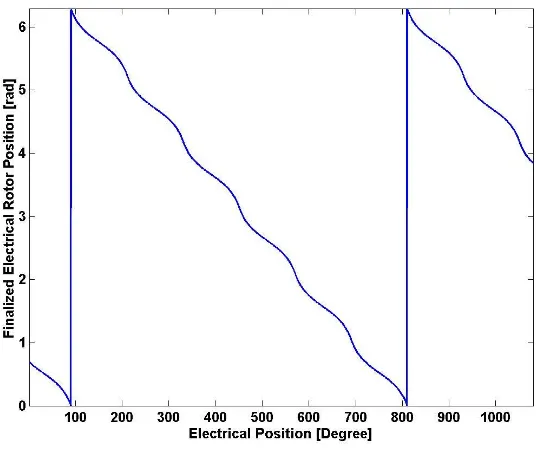
Fig. 3.5 shows that these three repetitive cases which are in the range of 0 to 360 degrees, can be manipulated to be 0 to 180 degrees (π rad) in one period as calculated

in (3.20). The manipulated electrical rotor position is normalized and depicted in Fig. 3.6. Finally, two periods of the manipulated position are combined to be a period of

the calculated electrical rotor position (_cal) in the range of 0 to 2π rad (360 degrees) as plotted in Fig. 3.7. Even though the calculated electrical rotor position is in the regular range, an uncertainty of magnet poles (±180 degree) has not been taken into account. The uncertainty can lead to drive the machine in an opposite direction.

( ) , ( ) ( ): case1 18 2

5

( ) , ( ) ( ): case2 18 6

( ) , ( ) ( ): case3 18 6

cal

v w

u v u w

u w u

v u v w

v u v

w u w v

w

 



 



 _ _ _{  }

 

 

_     

 

 _ _ _{ } _



(46)

Fig. 3.6: Manipulated calculated electrical rotor position

Fig. 3.7: DFC electrical rotor position (αcal)

3.2 DFC Implementation

(47)

a. PMSM1

PMSM1 is a small PMSM, has an out rotor with 12 permanent magnets and 9 stator teeth with a machine neutral point accessible. The electrical power of PMSM1 is 7.5 W, approximately. The PMSM1 is depicted in Fig. 3.8.

Fig. 3.8: PMSM1

b. PMSM2

PMSM2 is a bigger motor than PMSM1, consists of an out rotor with 20 permanent magnet pole pairs (40 permanent magnets) and 54 stator teeth with a machine neutral point accessible. The blank area inside the motor as in Fig. 3.9, was used for a Hall sensor which has been removed. The PMSM2 power is 712 W, approximately.

(48)

c. PMSM3

PMSM3 has a different structure, when compared to PMSM1 and PMSM2. The magnets are buried inside the rotor, which is called non-salient poles PMSM or buried magnet PMSM. The power of PMSM3 is in the region of 3.7 kW. This machine has 9 stator teeth and 6 magnets.

Fig. 3.10: PMSM3

3.2.1 Software Implementation

Generally, there are two parts, i.e. a machine model and a drive circuit with programmable algorithms, which are required to do software simulation.

Consequently, Simulink is selected as a simulation environment to execute the DFC method with PMSM models. The machine models in Simulink are available only in synchronous frame (d,q) with constant phase inductance values and without the machine neutral point. Thus, a new PMSM model with nonlinear phase inductance characteristics and the neutral point accessibility has to be designed. In [26] and [27], the saturation of the lamination core has been implemented into machine models, which are represented by coefficients instead of the nonlinear magnetization (BH)

(49)

For that reason, the nonlinear BH curve for the inductance and the neutral point have to be added into the model. Due to that, the mutual inductances between phases or the coupled flux of other phases as shown in the DFC calculation cannot be neglected. Therefore, it leads to the difficulty to model the machine to react as the real PMSM in Simulink.

A solution to overcome the mentioned obstacles is to use a finite element method (FEM) as in [28 – 30]. A cooperative simulation with Simplorer and Maxwell is selected. Maxwell can compute many kinds of calculations by FEM and many values

e.g. the flux density and the inductance, which cannot be measured and extracted in other simulation environments. Even signals which are difficult to obtain from real

machines can be attained. The nonlinear BH curve can be included into the machine model. Nevertheless, all machine data and properties, i.e. defining coil terminals, group coil terminals to phase windings, the permanent magnets properties, allocation of material properties and magnets including the BH curve of the lamination stack, the rotor and the stator lamination stack geometry, and assign the excitation direction, are required. Otherwise, the machine model cannot behave as the real machine.

For Simplorer, the co-simulation with Maxwell is available and many relevant parts, i.e. the drive system, the measuring system, the modulation algorithm, and extra programs in C language, can be added.

The simulation environment of the complete combination between Simplorer and Maxwell from Simplorer is shown in Fig. 3.11.

From Fig. 3.11, the DFC method with the modulation algorithm is programmed in C by the built in C editor and the PMSM model is linked to the PMSM modeled in Maxwell. This environment is firstly investigated in [31]. There are two inputs, i.e. a DFC input and a load. The DFC input is a maximum duty cycle of the PWM unit in percentage, which is used to generate the voltage vector. The load is another machine,

(50)

Fig. 3.11: Combination of software environments

According to the machine models, all three machines, i.e. PMSM1, PMSM2, and PMSM3, 2 dimensional (2D) models have been achieved in Maxwell as illustrated in

Fig. 3.12. However, only data and all properties of PMSM2 are available. Therefore, the PMSM2 model is validated and experimented. It is worth to mention that 3D models can be also implemented in Maxwell. Due to the high computational complexity of the 3D model, the 2D model is selected.

a) PMSM1 model b) PMSM2 model c) PMSM3 model

Fig. 3.12: 2D PMSM Model

PMSM

Model

(51)

After modeled and setup PMSM2, the model has to be validated to confirm its behaviors to be similar to the real PMSM2. Therefore, a no load running test is applied to examine both the real PMSM2 and the modeled PMSM2. Both are driven at 214 rounds per minute (rpm) and line to line induced voltages (VUV) are measured,

which are depicted in Fig. 3.13. The VUV signals have the same contents, i.e.

frequency, amplitude, and shape, except a little distortion on the FEM model signal. This is because the simulation sampling time is set to the maximum possible value (1 μs) to optimize the computational complexity. Hence, the PMSM2 model has the

correct characteristics as the real PMSM2.

a) Machine line to line induced voltage b) FEM model line to line induce voltage

Fig. 3.13: FEM model validation

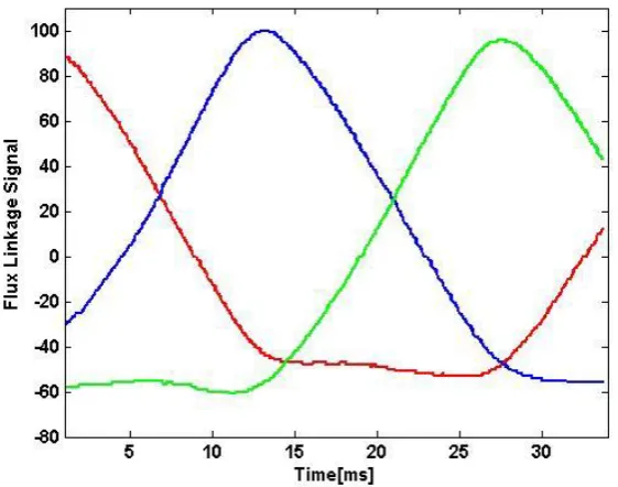
Subsequently, there are two experiments, which are tested and investigated with the PMSM2 model. Firstly, 20% (the maximum duty cycle of the PWM unit, PM) is

applied as the DFC input and the experiment time duration is 60 ms. The experimental results are the flux linkage signals (u,v,w) and the calculated electrical rotor position (αcal) as depicted in Fig. 3.14.

Next, the PMSM2 model is driven by the load machine as the step input at 35 rpm, the experiment is performed for 35 ms. The DFC input is set to a small value e.g. 4% , because VNAN is required to measure and the applied input must be the short duty cycle

which does not have any influence to drive the PMSM. The flux linkage signals have been extracted and measured as shown in Fig. 3.15(a). αcal is compared with the ideal

(52)

a) Flux linkage signals (u: red, v: blue, w: green)

b) Calculated electrical rotor position (_cal)

(53)

b) Comparison of calculated electrical positions (αcal : blue, α: red)

(54)

According to the experimental results, the flux linkage signals can be extracted in both experiments. They are periodical signals with similar shape and each signal is phase shifted as three phase system. αcal can be also found. A period of αcalis from 0

to 360 degrees, which means that two periods of flux linkage signals are used. In this case, the PMSM2 has 40 rotor magnet poles. Hence, there are 40 periods of each phase flux linkage signal and 20 periods of calculated electrical rotor position for one mechanical revolution. The ideal electrical rotor position (α) and αcal are similar to

each other as in Fig. 3.15(b), except in the beginning. This is because αcal is related to

influence of the machine stator currents, which is not the same as the ideal position.

αcal is from 0 to 145 degrees, approximately. It conforms to the period of the flux

linkage signals, which is less than a period. It shows that the machine information can be found by DFC much more than with the mechanical sensors.

3.2.2 Hardware Implementation

All PMSMs are implemented on a real time controller based on a TriCore PXROS platform. The microcontroller is a TC1796 (32-bit TriCore™ Microcontrollers). The TCP/IP protocol is a communication protocol between the TriCore PXROS platform and a host computer. Each machine experimental setup and results are described as following.

3.2.2.1 PMSM1

PMSM1 is connected to the TriCore PXROS platform, where the driving circuit, an artificial neutral point circuit, and a very fast analog to digital converter (FADC) with 10 bits resolution and 280 ns conversion time are compacted as illustrated in Fig. 3.16. VDC for PMSM1 is 12 V and the frequency of the PWM unit is 20 kHz. The

motor is driven by a MOSFET power stage.

Moreover, the test bench for small machines is also designed in order to test other motors as shown in Fig. 3.17. The tested machine shaft is coupled to a load motor

(55)

Fig. 3.16: Connected PMSM1 with TriCore PXROS platform

Fig. 3.17: Test bench for small machines

(56)

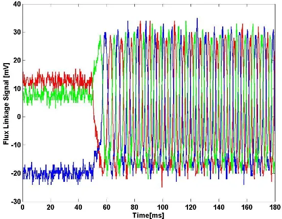
Two experiments are achieved. Firstly, a step input in Fig. 3.18 is applied as the DFC input, where PM is set at 10%. The time duration of the experiment is 180 ms. The

flux linkage signals (u,v,w) and the calculated electrical rotor position (_cal) are the experimental results, which are displayed in Fig. 3.19 (a) and (b), respectively.

(57)

The experimental results in Fig. 3.19 show that the flux linkage signals are changed, when the input is being changed. Furthermore, the flux linkage signals are also periodical signals as in the software implementation. αcal can be attained including

standstill from 0 to 50 ms.

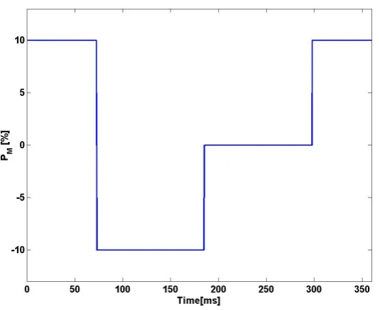
Next, the varied inputs, i.e. 10%, 0, and -10% are applied to drive PMSM1 as shown in Fig. 3.20. Each level is changed every 112.5 ms, which is a very small period. The main purpose of the experiment is to assure that the DFC method can obtain αcal for

all speeds, i.e. clockwise and anticlockwise directions, and at standstill. The results

are plotted in Fig. 3.21.

Fig. 3.20: Varied input pattern

Fig. 3.21 shows that the electrical rotor positions are obtained for all speeds and at standstill. The delay occurs whilst the direction is changed, because of the machine

(58)

position in Fig. 3.19 (b) and 3.21 (b), the directions are not the same while being applied the positive DFC input. It means that the uncertainty of rotor poles occurs in this case.

(59)

3.2.2.2 PMSM2

PMSM2 is also connected to the TriCore PXROS platform, but the driving circuit is not compacted with the system. A different inverter stack in the laboratory with IGBTs is selected to use. This is because the compacted system can deal only with two levels of the DC link voltage, i.e. 12 and 24 V. Therefore, a system with a wide range of the DC link voltage (VDC) is needed. The interface unit to use for the wide

range of the DC link voltage has been built and combined together with the TriCore PXROS platform in [32], which is called test bench for big machines as shown in Fig.

3.22. The voltage divider circuits and the artificial point circuits, which are suitable for higher DC link voltage levels i.e. 60, 200, and 400 V, are also designed.

Fig. 3.22: Test bench for big machines

PMSM2 is experimented in the same way as PMSM1. The PWM frequency is 10 kHz. 24 V is a required voltage level for PMSM2, but the DC link voltage is set to 30 V. This is because some voltages are dropped in the IGBT circuit. The applied varied input pattern is shown in Fig. 3.23. The experimental results are depicted in Fig. 3.24, which are similar to the PMSM1 experimental results in Fig. 3.21.

(60)

Fig. 3.23: Varied input pattern

(61)

b) Calculated electrical rotor position (_cal)

Fig. 3.24: Applied varied input experimental results

3.2.2.3 PMSM 3

PMSM3 is implemented on the same system as with PMSM2. The DC link voltage of PMSM3 is 200 V. Three levels of input (PM), 27%, 0, and -27%, are applied to drive

PMSM3. Each level is slightly changed by a