Please cite this article as: M. Mahdavi Jafari, G. R. Khayati, M. Hosseini, H. Danesh-Manesh, Modeling and Optimization of Roll-bonding Parameters for Bond Strength of Ti/Cu/Ti Clad Composites by Artificial Neural Networks and Genetic Algorithm, International Journal of Engineering (IJE), TRANSACTIONS C: Aspects Vol. 30, No. 12, (December 2017) 1885-1893
International Journal of Engineering
J o u r n a l H o m e p a g e : w w w . i j e . i rModeling and Optimization of Roll-bonding Parameters for Bond Strength of
Ti/Cu/Ti Clad Composites by Artificial Neural Networks and Genetic Algorithm
M. Mahdavi Jafaria, G. R. Khayati*a, M. Hosseinib,c, H. Danesh-Maneshc
a Department of Materials Science and Engineering, Shahid Bahonar University of Kerman, Kerman, Iran b Department of Mechanical Engineering, Faculty of Engineering, University of Hormozgan, Bandar Abbas, Iran c Department of Materials Science and Engineering, School of Engineering, Shiraz University, Shiraz, Iran
P A P E R I N F O
Paper history:
Received 02 April 2017
Received in revised form 30 July 2017 Accepted 08 September 2017
Keywords:
Ti/Cu/Ti Clad Composite Roll-bonding
Bond Strength Genetic Algorithm Artificial Neural Network
A B S T R A C T
This paper deals with modeling and optimization of the roll-bonding process of Ti/Cu/Ti composite for determination of the best roll-bonding parameters leading to the maximum Ti/Cu bond strength by combination of neural network and genetic algorithm. An artificial neural network (ANN) program has been proposed to determine the effect of practical parameters, i.e., rolling temperature, reduction in thickness, post-annealing time, post-annealing temperature and rolling speed on the bond strength of Ti/Cu composite. The most suitable model with correlation coefficient (R2) of 0.98 and mean absolute error (MAPE) 3.5 was determined using genetic algorithm (GA) and the optimum practice condition are proposed. Moreover, the sensitivity analysis results showed the post-annealing temperature with the negative effects is the most influential parameter on the strength of bonding.
doi: 10.5829/ije.2017.30.12c.10
1. INTRODUCTION1
Generally, cladding is the bonding of one metal over another as a coating to modify the surface properties of materials in engineering applications. The Ti/Cu/Ti is usually applied for high conductivity devices in corrosive environments, such as busbars for supplying current in the galvanizing lines, anode for chromium-plating and anode for the chloralkaline electrolysis [1].
Rutin method for cladding of Cu by Ti, i.e., indirect extrusion [2] and explosive welding [3] have some limitations, e.g., high temperature as well as limitation in shape and size of the sample. Roll bonding as an alternative method with unique advantages such as an efficient and economical method [4, 5]. In addition, one of the most characteristics of a clad composite is the stability of its bonds during the operation and manufacturing procedure. Generally, the bond strength in the rolling process is a function of time and temperature of pre- and post-annealing, rolling
*Corresponding Author’s Email: [email protected] (G. R. Khayati)
strength of Ti/Cu/Ti composite from entailed 37 experimental schedules; (b) optimizing process parameters by combining GA– ANN; (c) applying sensitivity analysis for determination of the most significant controlling parameters of the bond strength.
2. ARTIFICIAL NEURAL NETWORKS
ANN methods are based on some significant conceptions that have been provided by neuroscientists. In the ANN method, a simulation of a small part of the central nervous system is performed wherein stimulation data are fed to the input neurons (synapses), and these stimuli are adopted by weights (synaptic weights). The weights are balanced by an activation function, and results impute to the other neurons. All of the neurons are highly interconnected, and the activation values may be reported as results or may be fed to the next model. These connection weights are changed during training step to find the best generalization and interpolation of training patterns presented to the network during training to achieve the desired accuracy by the network. The most suitable architecture and nature of the neurons of the ANN are problem specific. ANNs have been applied for the range of goals, like constraint satisfaction, content addressable memories, control, data compression, diagnostics, forecasting, general mapping, optimization and pattern recognition [17].
2. 1. Multi-Layer Perceptron ANN Among
different types of ANNs (i.e., multilayer perceptron [MLP], Radial Basis [RB], Kohonen, probabilistic neural network [PNN] and generalized regression neural network [GRNN]), multilayer perceptron (MLP) neural networks are quite common and applied for the present work. In MLP networks, neurons are sorted in layers with connectivity between the neurons of various layers, i.e. input layer, hidden layer and output layer [18, 19]. For ANN modeling commonly three activation functions are used for the hidden and the output layers that are usually as hyperbolic tangent sigmoid (tansig), linear (purelin) and log-sigmoid (logsig). The error for hidden layers is specified by back-propagation algorithm [20]. During learning, the weights of the neurons are optimized according to the following phases:
Step 1. A training sample is provided to the neural network;
Step 2. The network’s output is evaluated with the desired output from sample. The error in each output neuron is determined;
Step 3. For each neuron, the output is determined, and a scaling parameter, how much lower or higher the output is adapted to match the desired output;
Step 4. The weight of the neurons is adapted to lower the local error;
Step 5. ‘‘Blame’’ for the local error is allocated to neurons at the previous level, giving high responsibility to neurons connected by stronger weights;
Step 6. Phases (3–5) are repeated on neurons on former level, using each one’s ‘‘blame’’ as error. Once a trained network sets up, new data from the same knowledge domain can be imported into the network and get good results.
2. 2. Selection of ANN Architecture To the best
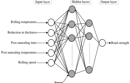
of our knowledge, the bond strength of Ti/Cu/Ti composites made by roll bonding is a function of rolling temperature, reduction in thickness, post-annealing time, post-annealing temperature and rolling speed. In this study, these parameters were selected as input variables in the ANN model while the bond strength of composite was the output value as shown in Figure 1. To develop a suitable ANN in the specific field, two main tasks were done; first, a data set of inputs and targets were prepared for training and testing of the network (Table 1). Also, each network was trained with 80% of the data and then tested by the other 20% of the data randomly selected from the data set. Second, a good architecture should be specified. In this study, MATLAB (version 2014b) based ANN toolbox was used to the ANN computing technique.
Defining the architecture of the network is a very important task because it affected the performance of the network. A program has been implemented in MATLAB® to evaluate various architectures of feed-forward back propagation ANN with several training algorithms such as Powell–Beale conjugate gradient algorithm (CGB), Levernberg-Marquardt algorithm (LM), scaled conjugate gradient algorithm (SCG) and quasi-Newton method (BFG) in one hidden layer to determine the one architecture with the lowest mean absolute percentage error (MAPE) for the testing data set.
Figure 1. Schematic description of artificial neural network configuration
Hidden layers Output layer
Bond strength
Neuron Rolling temperature
Reduction in thickness
Post-annealing time
Post-annealing temperature
TABLE 1. The statistical information of the developed datasets
Parameters
Input variable Maximum Minimum Average
Standard deviation
Rolling
temperature ( °C) 460 20 230.42 170.91 Reduction in
thickness (%) 62 44 52.86 7.04 Post-annealing
time (min) 200 30 99.43 65.87 Post-annealing
temperature (°C) 650 320 466 125.94 Rolling speed
(rpm) 12 3 7.18 3.32
Output variable
Bond strength
(N/mm) 20.95 8 14.82 3
The optimum configuration between the practical parameters and bond strength using ANNs were performed from data presented in Table 2. A four-fold loop was used in ANN to check all possible combinations of training algorithm, the transfer function of hidden and output layer and the number of neurons in the hidden layer.
The results of the ANN performance test were saved in a five-dimensional matrix. Then, at the end of the run, the program found the best architecture with the lowest MAPE in one hidden layer. Based on Kolmogorov’s theorem, it was demonstrated that at most four layers [21] could approximate any function.
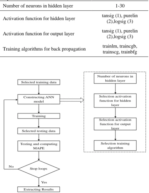
Therefore, different ANN structures in the range from a single layer up to three hidden layers were processed with characteristics of best architecture. The above-mentioned specifications are training algorithm and the transfer function in hidden layers and output layer. Figure 2 depicts the flowchart of the whole procedure.
3.GENETIC ALGORITHMS
Genetic algorithms are search algorithms proposed to mimic the principles of biological evolution in the natural genetic system. GAs are also known as stochastic sampling technique, as well as a method to solve complex processes such as multi-modal, discontinuous, non-differentiable, etc. These strategies keep and manipulate a population of solutions and use their search for better solutions based on ‘survival of the fittest’ method. GAs answer linear and nonlinear problems by exploring all regions of the stage space and exploiting candidate areas through mutation, crossover and selection processes used by individuals in the population.
TABLE 2. The ANN architecture variables in one hidden layer
Number of neurons in hidden layer 1-30
Activation function for hidden layer tansig (1), purelin (2),logsig (3)
Activation function for output layer tansig (1), purelin (2),logsig (3)
Training algorithms for back propagation trainlm, traincgb, trainscg, trainbfg
Figure 2. The flowchart of finding suitable the ANN architecture
Using the GAs, each individual in the population
requires being determined in a chromosome
representation [22]. A chromosome is made up of a sequence of genes from a specified alphabet. An alphabet could include binary digits, floating point numbers, integers, symbols and matrices. The representation method specifies how the problem is formed in the GA and defines the genetic operators that are applied. In this study, a chromosome is provided by a vector of floating point numbers with values within the variable upper and lower bonds, as it has been presented that natural representations are more effective and propose better solutions [22, 23].
In this case, the population size is 50 and the chromosome length represents the vector length of the solution to the problem; thus, each gene shows a variable of the problem. The genes values are forced to remain in the interval establish set by its variables, so the genetic operators must fulfill this requirement.
3. 1. Selection Selection of individuals plays an
important role in a GA. In selection individual values elected as ‘parents’. There are different selection methods. In this study, the roulette wheel selection in
Selected training data
Constructing ANN model
Number of neurons in hidden layer
Selection activation function for hidden
layer
Selection activation function for output
layer
Selection training algorithm Training
Extracting Results Testing and computing
MAPE Selected testing data
Stop loops No
which the area of each segment is proportional to its expectation was used. The algorithm then uses a random number to choose one of the sections with a probability equal to its area. Genetic operators are applied to generate offsprings in the next generation that differ from their parents, but maintain features of parents. There are many methods that these operators can be developed. Crossover and mutation are the most commonly used ways.
3. 2. Crossover Crossover is the recombination of
the information from two good parent solutions into what we expect are even better offspring solutions. The problem is to propose a crossover operator that considers features of both parent individuals. This means the two individuals are chosen randomly from the population and a crossover point is chosen randomly on the individuals. By exchanging the right part of crossover point of the two individuals, two new individuals are generated. The crossover process can generate new individuals i.e., different from the parents. The operation of proposed individuals determined during the searching extent. It reflects the ideology of information exchange in nature. In this study, the scattered crossover is applied. Scattered crossover generates a random binary vector. It then chooses the genes, where the vector is a 1 from the first parent and a 0 from the second parent, and combines the genes to create the child. The crossover rate is 90%, whereas the remaining 10% is added to the next generation without crossover.
3. 3. Mutation The mutation process includes
randomly modifying the value of each factor of the chromosome according to the mutation probability. Therefore, the searching scope can be expanded. In this study, the uniform mutation is applied. Uniform mutation is a two-phase process. First, the algorithm chooses a fraction of the vector entries of an individual for mutation, where each entry has a probability of mutation rate of being mutated. In the second phase, the algorithm replaces each selected entry by a random number selected uniformly from the range for that entry. If the mutation rate is too low, many binary bits that may be effective are never tried, but if it is too high, there will be much random perturbation, and the offspring will lose the useful information of the parents. The common value for the mutation rate is 1%.
4. INTEGRATION OF GA AND ANN
The outline of the above optimization algorithm is shown in Figure 3. Accordingly, the program for the process optimization of roll bonding has been developed using MATLAB. The optimization technique of this model is introduced as follows:
(1) The combined ANN/GA method creates an initial population of chromosomes (candidate solutions to the problem) from the first generation.
(2) The fitness f(x) of each of the chromosome in the population is determined.
(3) A population for the next generation is generated by the genetic processes (crossover and mutation). These processes are applied to the chromosomes in a formal generation with the probabilities according to their fitness.
(4) A new generation of roll bonding conditions is created. This algorithm is repeated to breed next generation. Finally, the population will move to the condition that corresponds to the maximum value of bond strength.
(5) The above phases are repeated until the termination factor has been satisfied. Once the GA is done over 200 iterations or the fitness function was equal 20.9, the evolution of the generation would be finished
5. RESULTS AND DISCUSSION
5. 1. ANN Model Results According to Table 3,
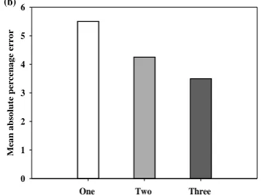
the results of the program in one hidden layer showed that the best architecture obtained by SCG training algorithm. The best architecture in one hidden layer has logsig transfer function in hidden layer and purelin transfer function in output layer and the lowest MAPE with this transfer function in hidden layer and output layer obtained by three hidden layers as seen in Figure 4.
Figure 3. Flowchart of optimization process based on ANN and GA
Start
Create initial random population
Perform ANN simulation
Fitness function evaluation
Selection
Crossover
Mutation Stop criterion
No Report result
This result indicates that to describe the complex relationship between the bond strength of Ti and Cu layers in the Ti/Cu/Ti composites and chosen input parameters requires a more complicated architecture.
TABLE 3. Lowest MAPE for each training algorithm
Algorithm LM CGB SCG BFG
Mean absolute percentage error 7.2 6.5 5.5 5.8
Figure4. Lowest MAPE in each transfer function in (a) one hidden layer and (b) whole one, two and three hidden layers.
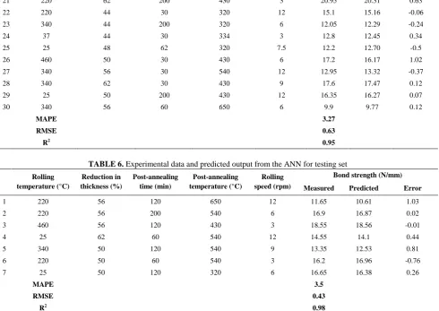
Characteristics of prime architecture are abbreviated in Table 4. The predicted values, deviation and percentage error of bond strength are abbreviated in Tables 5 and 6. The accuracy of the ANN was tested using the test values (Table 6) selected from the experimental results that were not applied during the learning process.
TABLE 4. Specifications of prime architecture
Training algorithm Layer no Neuron no. Transfer function
Layer #1 Layer #2 Layer #3 Layer #4 Layer #1 Layer #2 Layer #3 Layer #4
SCG 4 17 5 3 1 Logsig Logsig Logsig Purelin
TABLE 5. Experimental data and predicted output from the ANN for training set
Rolling temperature (°C)
Reduction in thickness (%)
Post-annealing time (min)
Post-annealing temperature (°C)
Rolling speed (rpm)
Bond strength (N/mm)
Measured Predicted Error
1 25 56 30 320 3 18.35 `16.42 1.92
2 220 44 60 430 6 19.75 19.17 0.57
3 340 44 120 430 12 16.8 17.21 -0.41
4 460 62 200 650 12 10.8 10.62 0.17
5 25 56 60 430 9 19.45 18.29 1.15
6 220 50 30 650 9 11.2 11.47 -0.27
7 340 50 200 650 3 13.75 13.52 0.22
8 460 62 120 540 6 13.3 13.54 -0.24
9 25 44 120 650 3 12.5 12.34 0.15
10 460 44 30 540 3 12.5 12.29 0.20
11 20 44 30 339 6 12.2 11.83 0.36
12 460 50 60 320 12 14.5 14.71 -0.21
13 25 44 200 540 9 13.75 12.27 1.47
14 220 62 120 320 9 17.8 18.32 -0.52
15 340 62 60 320 3 17.05 17.97 -0.92
16 460 44 60 650 9 8 8.42 -0.42
17 25 62 30 650 6 12.7 13.66 -0.96
18 25 62 80 370 5.5 16.9 17.23 -0.33
19 58.5 62 197 359 3.5 17.4 17.75 -0.35
0 2 4 6 8 10 12 14 16 18 20
0 1
2 3
4
0 1 2 3
M
ean absolute
pe
rc
ent
age
e
rr
or
Transf
er fun
ction i n out
put l
ayer
Transfer function for hidden layer (a)
One Two Three
M
e
an absolute
pe
r
c
e
nag
e
e
r
r
or
0 1 2 3 4 5 6
20 460 56 200 320 9 14.95 15.26 -0.31
21 220 62 200 430 3 20.95 20.31 0.63
22 220 44 30 320 12 15.1 15.16 -0.06
23 340 44 200 320 6 12.05 12.29 -0.24
24 37 44 30 334 3 12.8 12.45 0.34
25 25 48 62 320 7.5 12.2 12.70 -0.5
26 460 50 30 430 6 17.2 16.17 1.02
27 340 56 30 540 12 12.95 13.32 -0.37
28 340 62 30 430 9 17.6 17.47 0.12
29 25 50 200 430 12 16.35 16.27 0.07
30 340 56 60 650 6 9.9 9.77 0.12
MAPE 3.27
RMSE 0.63
R2 0.95
TABLE 6. Experimental data and predicted output from the ANN for testing set
Rolling temperature (°C)
Reduction in thickness (%)
Post-annealing time (min)
Post-annealing temperature (°C)
Rolling speed (rpm)
Bond strength (N/mm)
Measured Predicted Error
1 220 56 120 650 12 11.65 10.61 1.03
2 220 56 200 540 6 16.9 16.87 0.02
3 460 56 120 430 3 18.55 18.56 -0.01
4 25 62 60 540 12 14.55 14.1 0.44
5 340 50 120 540 9 13.35 12.53 0.81
6 220 50 60 540 3 16.2 16.96 -0.76
7 25 50 120 320 6 16.65 16.38 0.26
MAPE 3.5
RMSE 0.43
R2 0.98
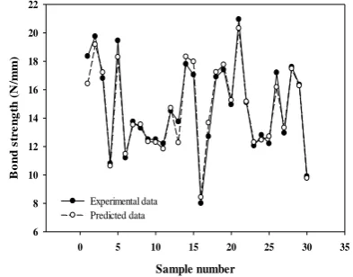
Figure 5 shows the comparison between the real and predicted values of test and training data. The results showed that the accuracy of the neural network is higher than 3.5%. However, several values were not as close as the others, which were related to the errors caused by the materials, the measurements and practical parameters.
5. 2. Sensitivity Analysis To determine the
relative significance of each parameter, the sensitivity analysis was applied. According to sensitivity analysis, it was possible to reduce the number of input parameters that do not have significant effect on performance of the model. In this case, the unnecessary data collected have been removed and significant cost reduction has been produced. A step-by-step process was developed on the trained ANN by charging each of the input factors, one at a time, at a constant rate.
Various constant rates (5, 10, 20) were selected in this study. The sensitivity of each input parameter was calculated by the following equation:
(1)
where Si (%) is the sensitivity level of an input
parameter and N (= 7) the number of datasets applied for sensitivity analyses. Figure 6 illustrates the sensitivity of variations for the bonding strength at each of the input variables. Accordingly, the post-annealing temperature is the most significant parameter followed by the reduction in thickness, rolling speed, rolling temperature and post annealing time. Similar results has been reported in the case of Taguchi analysis of the Ti/Cu/Ti bonding strength [24]. The significance of the post-annealing temperature is because of its influence on the weld toughness increment, residual stress reduction and atomic diffusion across the Cu/Ti interface [24].
Regarding Figure 6, another strongly effective parameter is the reduction in thickness. Considering the film theory, it has been shown that an increment on the reduction in thickness increases the bonding area via the
formation of larger surface cracks, and consequently
1
1
%
100
%
N
i
j
j
changein output
S
N
changeininput
higher content of the extruded virgin metals (which has the critical roles in the joint formation during the roll-bonding of similar or dissimilar metallic materials) [25].
5. 3. Genetic Algorithm Results The GA run was
carried out to find the optimum practical parameters of roll bonding process for the highest bond strength. The GA has reached the maximum value after the end of 43 interactions. The two last chromosomes have recorded the final optimum results. The predicted optimum process condition by GA is further validated by producing two samples of Ti/Cu/Ti composite under the proposed optimum conditions. Table 7 shows the comparison of ANN predicted and experimental values of bond strength. From Table 7, it is clear that sample 2 had higher bond strength compared to sample 1.
The comparison of the proposed optimum condition of GA-ANN for maximum bond strength is presented in Table 8.
Figure 5. Analogy of experimental and predicted bond strength for training and testing prime model
Figure6. The significance of input variables in bond strength
It can be concluded from Table 8 that combined GA– ANN algorithm is a powerful and efficient model to find the optimum conditions for producing Ti/Cu/Ti clad composite with the maximum bond strength.
TABLE 7. The optimum process parameters for roll bonding obtained from GA
Rolling
temperature (°C)
Reduction in thickness (%)
Post-annealing time (min)
Post-annealing temperature (°C)
Rolling speed (rpm)
Bond strength (N/mm)
Measured Predicted
54.93 58.12 189.8 449.09 7.74 20.09 19.30
102.78 54.83 172.6 400.11 7.45 20.80 20.40
TABLE 8. Bond strength of Cu/Ti layers under the initial and optimal process parameters
Process parameters Initial condition Optimized condition Improvement (%)
Rolling temperature (°C) 220 102.78 53
Reduction in thickness (%) 62 54.83 11.5
Post-annealing time (min) 200 172.6 14
Post-annealing temperature (°C) 430 400.11 7
Rolling speed (rpm) 3 7.45 148.5
Bond strength (N/mm) 20.95 20.4
Sample number
0 5 10 15 20 25 30 35
B
o
n
d
s
tr
e
n
g
th
(
N
/m
m
)
6 8 10 12 14 16 18 20 22
Experimental data Predicted data
Sample number
0 1 2 3 4 5 6 7 8
B
o
n
d
s
tr
e
n
g
th
(
N
/m
m
)
10 12 14 16 18 20
Experimental data Predicted data
-10 -8 -6 -4 -2 0 2 4 6 8 10
Rolling temperature (°C)
Post-annealing temperature (°C)
Reduction in thickness (%)
Rolling speed (rpm)
Post-annealing time (min)
Sens
iti
vity
le
vel
+5% -5%
6. CONCLUSION
The following conclusions are drawn from this work. 1. The ANN model with three hidden layers with 17, 5 and 2 neurons, respectively in each hidden layer is a useful method for the prediction of bond strength in Ti/Cu/Ti clad composite made by roll-bonding.
2. The combined GA–ANN algorithm was an effective model for optimizing roll-bonding parameters leading to the maximum of bond strength in Ti/Cu/Ti clad composite.
3. Sensitivity analysis showed that post-annealing temperature and reduction in thickness were the most significant parameter and post-annealing temperature was the most important parameter.
7. REFERENCES
1. Hosseini, M., Manesh, H.D. and Eizadjou, M., "Development of high-strength, good-conductivity Cu/Ti bulk nano-layered composites by a combined roll-bonding process", Journal of Alloys and Compounds, Vol. 701, No., (2017), 127-130. 2. Lee, J., Son, H., Oh, I., Kang, C., Yun, C., Lim, S. and Kwon,
H., "Fabrication and characterization of Ti–Cu clad materials by indirect extrusion", Journal of Materials Processing Technology, Vol. 187, No., (2007), 653-656.
3. Kahraman, N. and Gülenç, B., "Microstructural and mechanical properties of Cu–Ti plates bonded through explosive welding process", Journal of Materials Processing Technology, Vol. 169, No. 1, (2005), 67-71.
4. Hosseini, M., Yazdani, A. and Manesh, H.D., "Al 5083/sic p composites produced by continual annealing and roll-bonding",
Materials Science and Engineering: A, Vol. 585, (2013), 415-421.
5. Li, L., Nagai, K. and Yin, F., "Progress in cold roll bonding of metals", Science and Technology of Advanced Materials, Vol. 9, No. 2, (2008), 023001.
6. Manesh, H.D. and Shahabi, H.S., "Effective parameters on bonding strength of roll bonded al/st/al multilayer strips",
Journal of Alloys and Compounds, Vol. 476, No. 1, (2009), 292-299.
7. Kalidass, S. and Ravikumar, T.M., "Cutting force prediction in end milling process of aisi 304 steel using solid carbide tools",
International Journal of Engineering-Transactions A: Basics, Vol. 28, No. 7, (2015), 1074-1081.
8. Jiang, Z., Gyurova, L., Zhang, Z., Friedrich, K. and Schlarb, A.K., "Neural network based prediction on mechanical and wear properties of short fibers reinforced polyamide composites",
Materials & Design, Vol. 29, No. 3, (2008), 628-637.
9. Mahdavi Jafari, M. and Khayati, G.R., "Artificial neural network based prediction hardness of al2024-multiwall carbon nanotube composite prepared by mechanical alloying", International Journal of Engineering (IJE), Transactions C: Aspetcs, Vol. 29, No. 12, (2016), 1726-1733.
10. Kalantari, Z. and Razzaghi, M., " Predicting the buckling
capacity of steel cylindrical shells with rectangular stringers under axial loading by using artificial neural networks",
International Journal of Engineering-Transactions B: Applications, Vol. 28, No. 8, (2015), 1154-1163.
11. Ramana, K., Anita, T., Mandal, S., Kaliappan, S., Shaikh, H., Sivaprasad, P., Dayal, R. and Khatak, H., "Effect of different environmental parameters on pitting behavior of aisi type 316l stainless steel: Experimental studies and neural network modeling", Materials & Design, Vol. 30, No. 9, (2009), 3770-3775.
12. Ates, H., "Prediction of gas metal arc welding parameters based on artificial neural networks", Materials & Design, Vol. 28, No. 7, (2007), 2015-2023.
13. Babaei, H., "Prediction of deformation of circular plates subjected to impulsive loading using gmdh-type neural network", International Journal of Engineering-Transactions A: Basics, Vol. 27, No. 10, (2014), 1635-1644.
14. Zhang, X.-J., Chen, K.-Z. and Feng, X.-A., "Material selection using an improved genetic algorithm for material design of components made of a multiphase material", Materials & Design, Vol. 29, No. 5, (2008), 972-981.
15. Sousa, L., Castro, C. and Antonio, C., "Optimal design of v and u bending processes using genetic algorithms", Journal of Materials Processing Technology, Vol. 172, No. 1, (2006), 35-41.
16. Tsoukalas, V., "Optimization of porosity formation in alsi 9 cu 3 pressure die castings using genetic algorithm analysis",
Materials & Design, Vol. 29, No. 10, (2008), 2027-2033. 17. Zhang, Z. and Friedrich, K., "Artificial neural networks applied
to polymer composites: A review", Composites Science and technology, Vol. 63, No. 14, (2003), 2029-2044.
18. Chun, M., Biglou, J., Lenard, J. and Kim, J., "Using neural networks to predict parameters in the hot working of aluminum alloys", Journal of Materials Processing Technology, Vol. 86, No. 1, (1999), 245-251.
19. Anijdan, S.M. and Bahrami, A., "A new method in prediction of tcp phases formation in superalloys", Materials Science and Engineering: A, Vol. 396, No. 1, (2005), 138-142.
20. Mahdavi Jafari, M., Soroushian, S. and Khayati, G.R., "Hardness optimization for al6061-mwcnt nanocomposite prepared by mechanical alloying using artificial neural networks and genetic algorithm", Journal of Ultrafine Grained and Nanostructured Materials, Vol. 50, No. 1, (2017), 23-32. 21. Murtagh, F., "Multilayer perceptrons for classification and
regression", Neurocomputing, Vol. 2, No. 5, (1991), 183-197. 22. Anijdan, S.M., Madaah-Hosseini, H. and Bahrami, A., "Flow
stress optimization for 304 stainless steel under cold and warm compression by artificial neural network and genetic algorithm",
Materials & Design, Vol. 28, No. 2, (2007), 609-615.
23. Blanco, A., Delgado, M. and Pegalajar, M.C., "A real-coded genetic algorithm for training recurrent neural networks",
Neural Networks, Vol. 14, No. 1, (2001), 93-105.
24. Hosseini, M. and Manesh, H.D., "Bond strength optimization of ti/cu/ti clad composites produced by roll-bonding", Materials & Design, Vol. 81, (2015), 122-132.
Modeling and Optimization of Roll-bonding Parameters for Bond Strength of
Ti/Cu/Ti Clad Composites by Artificial Neural Networks and Genetic Algorithm
M. Mahdavi Jafaria, G. R. Khayati*a, M. Hosseinib,c, H. Danesh-Maneshc
a Department of Materials Science and Engineering, Shahid Bahonar University of Kerman, Kerman, Iran. b Department of Mechanical Engineering, Faculty of Engineering, University of Hormozgan, Bandar Abbas, Iran c Department of Materials Science and Engineering, School of Engineering, Shiraz University, Shiraz, Iran
P A P E R I N F O
Paper history:
Received 02 April 2017
Received in revised form 30 July 2017 Accepted 08 September 2017
Keywords:
Ti/Cu/Ti Clad Composite Roll-bonding
Bond Strength Genetic Algorithm Artificial Neural Network
ديكچ ه ای ن هلاقم هب لدم زاس ی و نهب ی ه زاس ی ارف ی دن لاصتا درون ی زوپماک ی ت Ti/Cu/Ti
عت فده اب یی ن اهرتماراپ ی هب ی هن تهج ازفا ی ش پ ماکحتسا ی دنو کرت زا هدافتسا اب ی
ب بصع هکبش ی روگلا و ی مت تنژ ی ک م ی دزادرپ . همانرب ا ی زا هکبش ی بصع ی عونصم ی ( ANNs ارب ) ی عت یی ن اهرتماراپ رثا یی ظن ی ر امد ی راکبات نامز ،تماخض رد شهاک ،درون ی لوا ی ،ه امد ی راکبات ی لوا ی ه ور رب درون تعرس و ی پ ماکحتسا ی دنو زوپماک ی ت Ti/Cu/Ti پ ی داهنش درگ ی د رتهب . ی ن رض اب لدم ی ب حصت ی ح ( R2 ) لداعم 0.98 و م ی گنا ی ن قلطم اطخ ( MAPE ) 3.5 عت یی ن و اب هدافتسا زا روگلا ی مت تنژ ی ک ( GA ) ارش ی ط هب ی هن پ ی داهنش دش . هولاع رب ا ی ،ن اتن ی ج لانآ ی ز ساسح ی ت ناشن داد هک امد ی راکبات ی لوا ی ه اب رثا فنم ی رتراذگرثا ی ن لماع رب ماکحتسا پ ی دنو تسا .