AN INTELLIGENT SYSTEM’S APPROACH FOR
REVITALIZATION OF BROWN FIELDS USING ONLY
PRODUCTION RATE DATA
S.D. Mohaghegh*and R. Gaskari
Department of Petroleum and Natural Gas Engineering, West Virginia University P.O. Box 6070, Morgantown, U.S.A.
[email protected] - [email protected]
*Corresponding Author
(Received: February 22, 2007 – Accepted in Revised Form: September 25, 2008)
Abstract State-of-the-art data analysis in production allows engineers to characterize reservoirs using production data. This saves companies large sums that should otherwise be spend on well testing and reservoir simulation and modeling. There are two shortcomings with today’s production data analysis: It needs bottom-hole or well-head pressure data in addition to data for rating reservoirs’ characterization. Analysis remains at the individual well level. It does not offer integration of results from individual wells to create a field-wide analysis.A new technique called Intelligent Production Data Analysis, IPDA, addresses both of these short-comings. Through an iterative technique, IPDA integrates Decline Curve Analysis, Type Curve Matching, and Numerical Reservoir Simulation (History Matching) in order to converge to a set of reservoir characteristics, compatible with all three techniques.Furthermore, once reservoir characteristics for individual wells in the field are identified through above process, and by using a unique Fuzzy Pattern Recognition technology the results are mapped on the entire field in order to evaluate reserve estimates, pin-point optimum infill drilling locations, track fluid flow and depletion, remaining reserves and finally identify under-performer wells.
Keywords Production Data, Mature Fields, Brown Fields, Reservoir Characterization
ﻩﺪﻴﻜﭼ
ﺵﻭﺭﻩﺩﺍﺩﯽﺳﺭﺮﺑﻦﻳﻮﻧﯼﺎﻫ
ﯽﮔﮋﻳﻭ ﻪﺑﯽﺑﺎﻴﺘﺳﺩ،ﺪﻴﻟﻮﺗﯼﺎﻫ
ﺩﺍﺩﺯﺍﻩﺩﺎﻔﺘﺳﺍﺎﺑﺍﺭﻥﺰﺨﻣﯼﺎﻫ
ﻩ
ﺪﻴﻟﻮﺗﯼﺎﻫ
ﯽﻣﻦﮑﻤﻣ
ﺩﺯﺎﺳ .
ﺵﻭﺭﻦﻳﺍﺯﺍﻩﺩﺎﻔﺘﺳﺍ
ﻪﻨﻳﺰﻫﺭﺩﯽﻳﻮﺟﻪﻓﺮﺻﺚﻋﺎﺑﺎﻫ
ﻩﺎﭼﺖﻔﮕﻨﻫﯼﺎﻫ
ﻪﻴﺒﺷﻭﯽﻳﺎﻣﺯﺁ
ﻥﺰﺨﻣﯼﺯﺎﺳ
ﯽﻣ ﺩﺩﺮﮔ .
ﺵﻭﺭ ﺭﺩ،ﻩﺪﻤﻋﻒﻌﺿﻭﺩ
ﻩﺩﺍﺩﯽﺳﺭﺮﺑﺩﻮﺟﻮﻣﯼﺎﻫ
ﯼﺎﻫ
ﺵﻭﺭ ﻦﻳﺍﺯﺎﻴﻧ،ﺪﻴﻟﻮﺗ
ﺎﻳﯽﻫﺎﭼﺮﺳﺭﺎﺸﻓﻪﺑﺎﻫ
ﻥﺪﺷﺩﻭﺪﺤﻣﺰﻴﻧ ﻭﯽﻫﺎﭼ ﻪﺗ
ﻪﻴﺒﺷ ﯼﺯﺎﺳ
ﻩﺎﭼﻪﺑ
ﯽﻣﺩﺮﻔﻨﻣﯼﺎﻫ
ﺪﺷﺎﺑ .
ﺵﻭﺭﻦﻳﺍ
ﻂﺴﺑﯼﺍﺮﺑﯽﻧﺎﮑﻣﺍ ﻪﻧﻮﮔﭻﻴﻫﺎﻫ
ﺪﻧﺭﺍﺪﻧ ﻥﺰﺨﻣ ﻊﻣﺎﺟﻞﻴﻠﺤﺗ ﻪﺑﻥﺪﺷ ﻩﺩﺍﺩ
.
ﻡﺎﻧﻪﺑ ،ﻩﺪﺷ ﻪﺋﺍﺭﺍ ﺪﻳﺪﺟ ﺵﻭﺭ ﺭﺩ
"
ﻩﺩﺍﺩﺪﻨﻤﺷﻮﻫ ﯽﺳﺭﺮﺑ
ﺪﻴﻟﻮﺗ ﯼﺎﻫ
"
(IPDA)
ﻮﻣﺩﻮﺒﻤﮐ ﻭﺩ ﻦﻳﺍ
ﯽﻣﺭﺍﺮﻗ ﻪﺟﻮﺗ ﺩﺭ
ﺪﻧﺮﻴﮔ .
IPDA
ﯽﺳﺭﺮﺑ ﺵﻭﺭﻪﺳﻥﺩﺮﮐ ﺐﻴﮐﺮﺗﻪﻠﻴﺳﻭ ﻪﺑ
Decline
Curve
)
ﺪﻴﻟﻮﺗﺶﻫﺎﮐﯽﻨﺤﻨﻣ
( ، Type Curve Matching ﻭ
ﻪﻴﺒﺷ ﯼﺯﺎﺳ ﻩﺎﭼ
ﯽﮔﮋﻳﻭ ﻪﺑ ﯽﺑﺎﻴﺘﺳﺩ،ﻥﺰﺨﻣ ﯼﺎﻫ
ﯼﺎﻫ
ﯽﻣﻢﻫﺍﺮﻓﻕﻮﻓﺵﻭﺭﻪﺳﺮﻫﻪﺑﺖﺒﺴﻧ ﯼﺭﺎﮔﺯﺎﺳﺎﺑﺍﺭﻥﺰﺨﻣ
ﺩﺯﺎﺳ .
ﺮﺑ ﻩﻭﻼﻋ
ﯽﮔﮋﻳﻭﻪﺑﯽﺑﺎﻴﺘﺳﺩﺯﺍﺲﭘ،ﻦﻳﺍ
ﻫ ﯼﺎ ﻥﺰﺨﻣ ﺭﺩ ﻩﺎﭼ ﯼﺎﻫ
ﺪﺷﻩﺩﺍﺩﻂﺴﺑﻥﺰﺨﻣﻡﺎﻤﺗﻪﺑﻦﻴﺸﻴﭘﺞﻳﺎﺘﻧ،ﻥﺰﺨﻣﯼﻮﮕﻟﺍﯽﻳﺎﺳﺎﻨﺷﯼﺯﺎﻓﺵﻭﺭﻪﻠﻴﺳﻭﻪﺑ،ﺩﺮﻔﻨﻣ
ﯽﮔﮋﻳﻭﻦﻳﺍ ﻦﻴﻤﺨﺗﻭ
ﯽﻣﻦﮑﻤﻣﻥﺰﺨﻣﺮﺳﺍﺮﺳ ﺭﺩﺎﻫ
ﺩﺩﺮﮔ .
ﻪﻨﻴﻬﺑ ﺏﺎﺨﺘﻧﺍﻥﺎﮑﻣﺍ ﻞﻣﺎﺷﯼﺭﻭﺁ ﻦﻓﻦﻳﺍﯽﻳﺎﻬﻧﺞﻳﺎﺘﻧ
ﯼﺭﺎﻔﺣﻥﺎﮑﻣ
ﻩﺎﭼ ﯼﺎﻫ
ﺤﻣ،ﻥﺰﺨﻣﺭﺩﻝﺎﻴﺳﻥﺎﻳﺮﺟﺮﻴﺴﻣ ﯽﺳﺭﺮﺑ،ﯼﺪﻌﺑ
ﯽﻳﺎﺳﺎﻨﺷﻭﻥﺰﺨﻣﻩﺮﻴﺧﺫﻩﺪﻧﺎﻣﯽﻗﺎﺑﻪﺒﺳﺎ
ﻩﺎﭼ ﯼﺎﻫ
ﯽﻣﯽﻨﻴﺑﺶﻴﭘﺯﺍﺮﺘﻤﮐﯽﻳﺍﺭﺎﮐﺎﺑ
ﺪﺷﺎﺑ .
1. INTRODUCTION
Techniques of production data analysis (PDA) have improved significantly over the past several years. These techniques are used to provide information about reservoir permeability, fracture length, fracture conductivity, well drainage area,
through a software application [2].
Production data analysis techniques started systematically with a method presented by Arps in the 1950s [3]. Arps’ decline analysis, still being used because of its simplicity, is an empirical method that does not require any reservoir or well parameters. Arps’ equation is based on empirical relationships of rate vs time for oil wells and is shown below.
( )
b 1 t i bD 1 i q t q ⎟ ⎠ ⎞ ⎜ ⎝ ⎛ += (1)
In this relationship, b = 0 and b = 1 represent exponential and harmonic decline, respectively. Any value of b between 0 and 1 represents a hyperbolic decline. Although Arps’ equation is only for pseudo-steady state conditions, it has been often misused for oil and gas wells whose flow regimes are in a transient state.
Fetkovich, et al [4]proposed a set of equations described by exponent, b. The Fetkovich methodology analyzes oil wells producing at a constant pressure. He combined early time, analytical transient solutions with Arps’ equations for the later time, pseudo-steady state solutions. The Fetkovich method like Arps equation, calculates expected ultimate recovery.
Carter’s gas system type curves were published in 1985 [5]. Carter used a variable λ identifying the magnitude of the pressure drawdown in gas wells. A curve with a λ value of 1 corresponds to b = 0 in Fetkovich liquid decline curves and represents a liquid system curve with an exponential decline. Curves with λ = 0.5 and 0.75 are for gas wells with an increasing magnitude of pressure drawdown.
Agarwal [6] also introduced a method for production data analysis in 1999. This technique combines decline curve and type curve concepts for estimating reserves and other reservoir parameters for oil and gas wells using production data. Other methods were introduced by Fraim, et al [7], and Palacio, et al [8], which provides information on gas in place, permeability, and skin. There are also modern analytical methods that do not use type curves. One of these methods is “flowing material balance”. This technique provides
the hydrocarbons in place using production rate and flowing pressure data from a reservoir under volumetric depletion [6].
Today’s high prices have renewed focus on brown fields. Most of the fields that have been producing for many years have now become good candidates for infill drilling, re-fracturing or other operations that would revitalize these fields and turn them into profitable assets again. As engineers, geologists and managers start evaluating the potentials of these mature fields they encounter a hard and unforgiving reality. Production data (rate and not pressure data) is about the only data available for almost all wells. This fact limits the usability of most techniques that were mentioned in the previous paragraphs. Some wells here and there may have logs or even some pressure test data, but wells with such information usually belong to a small minority. Therefore, any evaluation made cannot be relied other than the existing production rate data.
Facing this reality, operators (or anyone performing the analysis on their behalf) are left with a limited set of choices. In this article we examine these choices, identify their strengths and limitations, recommend an alternative technique and demonstrate the benefits of the alternative technique using data from two fields. The first example is from the Golden Trend fields in Mid Continent of the United States. Wells in this field are operated by multiple operators are completed and producing from multiple formations such as Tulip Creek, 1st and 2nd Bromide, Viola, Sycamore, Hunton, Atoka, Chimney Hill and Mc Lish. The second example is a set of wells in the Wattenberg field producing from Codell and Niobrara formations in the D.J. Basin of Rockies.
regularly in the industry is Type Curve Matching. The strength of Type Curve Matching techniques is that it can provide reservoir characteristics such as permeability, drainage area and skin at the conclusion of analyses. The major problem with Type Curve Matching is the issue of subjectivity. In other words, the results of Type Curve Matching analysis are not repeatable. Production data from a particular well given to three engineers will produce three independent and sometime very different results. Figure 3 provides a realistic example.
The second limitation of Type Curve Matching analysis is the one it shares with Decline Curve Analysis, i.e. the results are well-based and there are no facilities to enable user to map the findings on the entire field or reservoir.
Another technique that is used for production data analysis but it is not as popular as Decline Curve Analysis or Type Curve Matching is the use of single-well radial reservoir simulators in order to perform history matching. This technique is not widely used for two reasons, specifically for mature fields and more specifically by independent produces. First, reservoir simulators are not known to be easily accessible at reasonable costs and their use are not as straight forward as Decline Curves or Type Curves. Secondly, history matching is not easy to perform and it takes a long time. Furthermore, even if the above two issues are overcome, the fact that history matching provides non-unique solutions, specifically when used for production data analysis remains and therefore, the technique suffers from the same subjectivity issues that has plagued the Type Curve Matching technique.
The new technique introduced here, namely Intelligent Production Data Analysis-IPDA, builds on the strength of the above three techniques and avoids their limitations. Furthermore, it introduces a new post-processing technology that capitalizes on the well-based information that is generated as a result of well by well production data analysis and maps these results on the entire field or reservoir. This post-processing technology is mainly a reservoir management tool that puts all the findings of production data analysis in perspective and allows managers and engineers to play “what-if” scenarios on their potential operations and make informed decisions.
2.INTELLIGENTPRODUCTIONDATA ANALYSIS-IPDA
As it was covered in the previous section, state-of-the-art data analysis in production leaves a lot to be desired when it comes to dealing with production rate data and especially when pressure data is not available, which is the case most of the times, when dealing with brown (mature) fields. The new technique that is being introduced here consists of two major components. The first component combines the three techniques mentioned above, namely Decline Curve Analysis, Type Curve Matching and Numerical Reservoir Simulation (history matching). The integration of these three techniques is accomplished through an iterative process that eventually converges to a set of reservoir characteristics for each well.
The second component of IPDA takes the results of the first component plus the location of each well, identified by their latitude and longitude, and deduces patterns that can help managers and engineers during the decision making process. This second component is accomplished through the use of a unique Fuzzy [9] Pattern Recognition technology. In the next two sections the details of each component will be discussed. Application of this technique on two mature fields follows the explanation of the methodology. This article is divided into two parts, each part dedicated to one of the components mentioned above.
2.1.
Part One: Intelligent Iterative Integrtion,
I
3The process has been named Intelligent Iterative Integration since it “Integrates” three techniques mentioned above (Decline Curve Analysis, Type Curve Matching and Numerical Reservoir Simulation). It accomplishes its task by using an “Iterative” process. And finally it used an automation approach that is only possible to accomplish through an “Intelligent” system’s technique. Figure 1 is the schematic diagram for the i3 process.
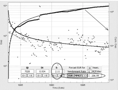
and the cumulative production versus time. This is demonstrated in Figure 2 for a well in the D. J. Basin. Initial production rate “Qi”, initial Decline rate “Di” and hyperbolic exponent “b” are automatically identified (note the value of b is 2.11). Furthermore, the 30 year Estimated Ultimate Recovery (EUR) is also calculated (note the value of EUR is 207 MMSCF).
The information generated as the result of Decline Curve Analysis is then passed on to a Type Curve Matching procedure. The appropriate type curves for the type of reservoir and fluid that is being investigated should be selected. For the purposes of this article the type curves developed by Cox, et al [11] was used since gas production from tight gas sands were being investigated. Figure 3 shows the actual production data from
the well shown in Figure 2. The actual production, plotted on a log-log scale, is on top of a series of type curves developed for the same value of hyperbolic exponent that has been found during the Decline Curve Analysis. Figure 4 shows the same production data plotted on a set of type curves for a different hyperbolic exponent (type curves in Figure 3 are developed for b = 2.11-same as the decline curves-and in Figure 4 developed for b = 1.5-different from the decline curves). Looking at the production data plotted in Figures 3 and 4, one can see that the data can be matched with any of the curves. This is a good
Figure 1. The intelligent iterative integration, i3 process.
Figure 2. Decline Curve Analysis of a well in the D. J. Basin.
Figure 3. Type curve matching with real production data is a
subjective process.
Figure 4. Type curve matching with real production data is a
example of the subjectivity of the Type Curve Matching procedure.
Assuming that we are happy with the results of Decline Curve Analysis (please note that the match achieved in the Decline Curve Analysis is subject to iterative modification and can be improved, the initial match is only a starting point) there are no reasons why we should not take advantage of the results of the Decline Curve Analysis in order to enhance the possibilities of success and removing the subjectivity from the Type Curve Matching procedure.
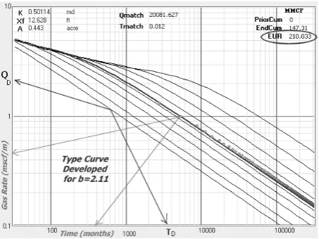
In Figure 5 we have taken full advantage of results of Decline Curve Analysis. We have done this by (A) plotting the production data that is result of Decline Curve Analysis rather than the actual production data. This model is much better behaved than the actual production data and can help us with a better and less subjective match. (B) By using the 30 Year EUR that was calculated from the Decline Curve Analysis for this well i.e. 207 MMSCF, as a guide we move the modeled data up and down and match it on different Xe/Xf curves until we get a calculated 30 Year EUR from the Type Curve Matching that is comparable to that of Decline Curve Analysis. For this particular well, as shown in Figure 5, the EUR is 210 MMSCF.
Once the match is completed the Type Curve Matching procedure provides us with permeability, fracture half length and drainage area. As part of the iterative process, if during the Type Curve
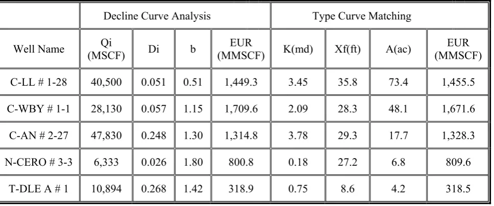
Matching procedure a good match cannot be achieved (a good match is defined as a match that not only looks reasonable during visual inspection but also provides reasonable values for the parameters while the EUR is reasonably close to that of the Decline Curve Analysis) we must go back to the Decline Curve Analysis and modify the match there in order to get a different “b” and EUR and also repeat the Type Curve Matching. If this practice brings us closer to a match that would satisfy both methods then we have moved (the modification of the Decline Curve Analysis) in the right direction and hopefully get a match if this practice has moved us farther away from a good match then we have to repeat the Decline Curve Analysis this time in the opposite direction. Our experience with this procedure shows that in most cases a single iteration achieves acceptable results. Table 1 shows the results of this process for five wells located in the Golden Trend fields of Oklahoma.
In order to complete the Type Curve Matching process knowledge about a set of parameters for the reservoir (field) being studied is required. These parameters are used during the calculation of permeability, fracture half length, drainage area and EUR. Following is the list of parameters that are required for Type Curve Matching procedure:
¾ Initial reservoir pressure; ¾ Average reservoir temperature; ¾ Gas specific gravity;
¾ Isotropicity (kx/ky ratio);
¾ Drainage shape factor (L/W ratio); ¾ Average porosity;
¾ Average pay thickness; ¾ Average gas saturation;
¾ Average flowing bottom-hole pressure. Most of the above parameters can be (and usually are) guessed within a particular range that is acceptable for a particular field. Usually the initial reservoir pressure for a field or formation is known within a reasonable range or it can be assumed based on formation depth. Formation depth can also be a good indication of average reservoir temperature. Gas specific gravity can be easily calculated based on the assumed average initial pressure and reservoir temperature. In most of our calculations we assume that the reservoir is
Figure 5. Type curve matching with modeled data is a less
isotropic, meaning that the kx/ky ratio is equal to 1. The drainage shape factor is also assumed to be 1 meaning that we are assuming a square drainage area. Average porosity, thickness and gas saturation can be calculated for each well from logs, if they are available. If they are not, then an average value for the entire field can be assumed. Intelligent Production Data Analysis-IPDA-allows for better matches and results with higher confidence level if wireline logs are available for the wells being analyzed. By having access to logs; porosity, thickness and saturation can be calculated and used individually for each well during the analysis. If and when such logs are not available or prove to be too expensive to analyze then the procedure allows the user to input an average value (as the best guess) for all wells.
The third and final step during the i3 process is numerical reservoir simulation. The reservoir simulation step itself is divided into two parts. First is the history matching and second is the Monte Carlo simulation. During history matching all the information that has been gathered during the Decline Curve Analysis and Type Curve Matching are used to initialize a single-well, radial numerical simulator. It is expected that some of the parameters that have been calculated during the Decline Curve Analysis and Type Curve Matching
(and are used as initial input to the simulator) be modified in order to achieve an acceptable match during the history matching process. If the modifications of one or several of these parameters prove to be very significant then the user must go back to the previous two techniques and modify them in the direction that would reduce the magnitude of the modifications in the history matching process. If the modifications are not significant then we can move to the next step. The question may rise that “what is considered to be significant?” This would be judgment call based on the available information and the parameters being modified. The rule of thumb would be that anywhere from 10 to 25 percent modification usually can be tolerated. The lower limit of this toleration would be for parameters with large magnitude and less uncertainty, such as initial pressure and the upper limit would be for parameters with small magnitude and more uncertainty such as permeability (given that we are analyzing wells in the tight gas reservoirs). Since we will be performing a Monte Carlo simulation in the next step certain amount of uncertainty can and will be tolerated. Figure 6 shows the results of history matching for a well in the Golden Trends.
Once a history match has been achieved, all the
TABLE 1. Reservoir Parameters and Eur Resulted from Integration of Decline Curve Analysis and Type Curve Matching.
Decline Curve Analysis Type Curve Matching
Well Name Qi
(MSCF) Di b
EUR
(MMSCF) K(md) Xf(ft) A(ac)
EUR (MMSCF) C-LL # 1-28 40,500 0.051 0.51 1,449.3 3.45 35.8 73.4 1,455.5 C-WBY # 1-1 28,130 0.057 1.15 1,709.6 2.09 28.3 48.1 1,671.6 C-AN # 2-27 47,830 0.248 1.30 1,314.8 3.78 29.3 17.7 1,328.3 N-CERO # 3-3 6,333 0.026 1.80 800.8 0.18 27.2 6.8 809.6
important parameters that are involved in the simulation process are assigned a probability distribution function (pdf) and the objective function (which is the history matched model) is run for 500 to 1000 times. Each time a run is completed the 30 year EUR is calculated and at the end they are plotted to form a “30 year EUR pdf”. Then the 30 year EUR values calculated from Decline Curve Analysis and Type Curve Matching are marked on the “30 year EUR pdf” plot. As long as the 30 year EUR values calculated from Decline Curve Analysis and Type Curve Matching are within the high frequency area of the plot, it means that results of the analysis are acceptable. Figure 7 shows the result of Monte Carlo simulation for the well that its history match is shown in Figure 6.
3.AUTOMATIONOFTHEPROCESS
Reading through the last section one might think that this procedure is hopelessly long and inefficient. This process has been automated in IPDA such that performing both Decline Curve
Analysis and Type Curve Matching procedure takes only a few seconds per well. The reservoir simulation process is currently being added to the automation process. The automation process that is being developed requires minimum interaction from the user.
3.1.
Part Two: Fuzzy Pattern Recognition for
Field-Wide Opportunity Identification
Oncethe i3 analysis for all the wells in a filed is completed, we have the following information for all the wells:
¾ Initial Flow Rate, Qi
¾ Initial Decline Rate, Di
¾ Hyperbolic exponent, b
¾ Permeability, k
¾ Drainage Area, A
¾ Fracture Half Length, Xf
¾ 30 Year Estimated Ultimate Recovery, EUR The objective of this segment of the analysis is to integrate all the above information in the context of the entire field in order to paint a picture on the status of the field, as it is now and to predict the
Figure 6. History match using a single-well radial reservoir simulator for
field status at any given time in future. Based on the picture that is being painted, and the changes that the field (reservoir) will go through as projected into future, this segment of the analysis allows engineers and managers to make business and engineering decisions that would maximize the return on the investment.
A set of Production Indicators (PI) are calculated for each well based on the rate versus time data. These Production Indicators simply provide a measure of each well’s production capability that might be used to compare them with the offset wells. Following is a list of Production Indicators that are automatically calculated for each well at the start of this procedure:
¾ Best 3, 6, 9 and 12 months of production ¾ First 3, 6, 9 and 12 months of production ¾ Three year cumulative production ¾ Five year cumulative production ¾ Ten year cumulative production ¾ Current cumulative production
Furthermore, results of Decline Curve Analysis are
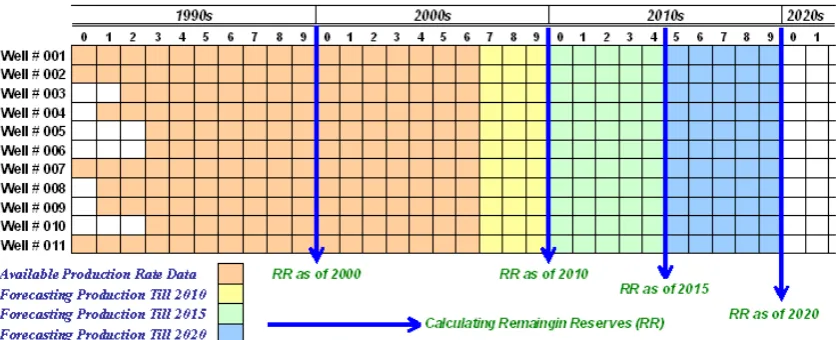
used in order to calculate the remaining reserves for each well. Remaining reserves is calculated based on 30 Year (or a different length of time) EUR from which the cumulative production has been subtracted. Figure 8 is a schematic diagram of how the Remaining Reserve is calculated for each well, since each well has a different starting date of production.
The Remaining Reserves can be calculated at different dates as shown by the arrows in Figure 8. Using this technique user can calculate:
¾ Remaining Reserves as of Today ¾ Remaining Reserves as of Year 2010 ¾ Remaining Reserves as of Year 2015
¾ Remaining Reserves as of Year 2020, and so on Using Fuzzy Pattern Recognition technology, IPDA deduces and generates two and three dimensional patterns and maps over the entire filed from the production indicators, the Remaining Reserves, and the data that was calculated during the i3 process. It also develops a set of Relative Reservoir Quality Indices based on the production
Figure 7. Results of Monte Carlo simulation with EUR as the objective
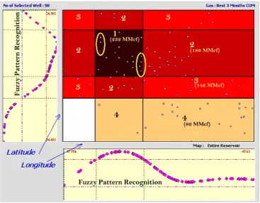
indicators and allow user to partition the filed into different reservoir qualities in order to identify sweet spots in the field. The collection of maps that are generated during this process will guide the engineers, geologists and managers in pin pointing the best infill locations in the filed and also identifying the under-performer wells that would be prime candidates for remedial operations such as re-stimulation and work-over. In this section application of this technology to two fields that were mentioned before is demonstrated and discussed. Figure 9 is an example of the 2D maps that are generated by IPDA. This figure includes a map (latitude vs. longitude) of the field showing the location of all the wells. Along the two axis of the map two graphs show the Production Indicator (last months of gas production in Figure 9) as a function of latitude and longitude.
Using Fuzzy Pattern Recognition a pattern is deduced in each graph (from the actual data). In each graph two separation lines separate high, medium and low values of PIs (last month production rate in this figure). As these separation lines intersect the fuzzy pattern curves vertical lines are generated that are then continued into the two dimensional map of the field. These vertical lines (from latitude and longitude) help to superimpose the high, medium and low separations of the PIs that were made at the latitude and longitude onto the 2D field map in order to delineate the field into different segments. The segments are then color coded to reflect the quality
of the reservoir. The darkness of the colors corresponds to higher quality of the reservoir. Different colors in the map represent different Relative Reservoir Quality Index (RRQI).
Figure 10 and 11 are two dimensional maps of some wells in the Golden Trend. This map includes 90 wells, operated by three different operators.
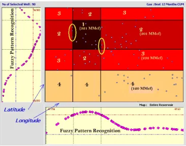
In Figure 10 the field has been partitioned based on the Best 3 Months of Production and in Figure 11 the field has been partitioned based on the Best 12 Months of Production. In these figures the Relative Reservoir Quality Index is identified for each region with a number from 1 to 5. A lower Relative Reservoir Quality Index means higher reservoir quality. For example in Figure 10 an average well in RRQI = 1 produces about 232 MMSCF while an average well in RRQI = 4 produces about 86 MMSCF during the Best 3 months of production. The Best 3 Months of Production for an average well in RRQI of 2 and 3 in this field are 186 and 142 MMSCF respectively. Figure 11 shows that an average well in RRQI = 1 produces about 321 MMSCF in its Best 12 Months while an average well in RRQI = 4 produces about 120 MMSCF in its Best 12 Months. The Best 12 Months of Production for an average well in RRQI of 2 and 3 are 301 and 232 MMSCF respectively.
Comparing Figures 10 and 11 one can see that as time goes on the size of the partitions change. Although all the partitions are relative (as the name
Figure 9. RRQI based on best 3 months of production.
suggests) more productive partitions usually get smaller as some wells move from higher productivity partitions to lower productivity partitions. For example the three wells in the left side of partition 1 during the Best 3 Months of production (Figure 11) move to a less productive partition (RRQI=2) during the partitioning of Best 12 Months of production (Figure 11). Same is true for four wells in the lower right corner of partition 1, Figure 11. These wells move to partitions with RRQI of 2 and 3 in Figure 11.
Movement of these wells from one partition to another can be an indication for relative reservoir depletion. Figure 12 shows the partitioning of the reservoir based on the last month production of each well. Although it seems that changes of well productivity along the latitude (the y axis) is relatively small, the change along the longitude (the x axis) is quite obvious. It can also be seen in the partitioning that the sweet spot (partition with RRQI=1) has moved further to the right of the field.
Also it is notable that in this field, the most productive part of the filed has an average
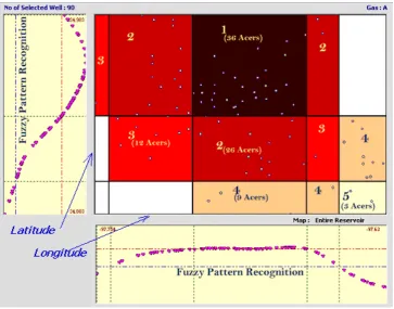
production that is more than 10 times as the least productive parts of the field. Figure 12 shows that an average well in the most productive partition of the filed can produce about 12.5 MMSCF/M while an average well in the least productive segments of the field would be producing about 1.2 MMCF/M. One of the parameters calculated during the i3 process was the Drainage Area. Figure 13 shows the application of Fuzzy Pattern Recognition to drainage area. This figure shows that better wells located in the north-central part of the field drain as much as 36 acres while least productive well, mainly in the south-eastern part of the field have an average drainage area of about 3 acres.
Figure 14 shows the three dimensional view of drainage area, fracture half length and permeability patterns developed in the Golden Trend due to production from 90 wells in the past several years. The patterns in this figure show the locations in the field that have higher values of permeability, that seem to be along the eastern and western edges of the field reducing from north to south while the drainage area and fracture half length behave in similar manner showing larger values toward the
Figure 12. RRQI based on last month production.
northern part of the field, specially on the eastern side.
Having such a view of the formation can help managers, geologists and engineers to develop strategies in further developing this field. Using the concept that was demonstrated in Figure 8 the Remaining Reserve in this filed is mapped and is shown in Figure 15. In this figure the Remaining Reserve is plotted as a function of time assuming no new wells are drilled.
Figure 16 shows the depletion in the reservoir from year 2005 to 2020 identifying portions of the field that would have remaining reserves that can be produced.
One can play “What If” scenarios by identifying locations in the field that are proposed as infill locations. Information from the off set wells are used through a neural network [12] modeling technique in order to estimate the decline behavior of the new location and the Remaining Reserve through time is recalculated as shown in Figure 16. The goal is to strategically place the infill wells in places where they would contribute to an efficient depletion of the reservoir.
Figure 17 shows the three dimensional view of drainage area, fracture half length and permeability patterns developed in the Wattenberg field producing from Codell and Niobrara formations in the D.J. Basin of Rockies. These three dimensional maps were developed from production of about 140 wells in the past several years. Please note that as the number of wells being analyzed in a particular filed increase, so does the resolution and accuracy of the maps developed using the Fuzzy Pattern Recognition technology. Using the concept that was demonstrated in Figure 8 the Remaining Reserve in the Wattenberg field is mapped and is shown in Figure 18. In this figure the Remaining Reserve is plotted as a function of time assuming no new wells are drilled.
Validation of the IPDA’s results as discussed in this article have been studied and are presented in two separate papers that are currently in print. In the first paper [13] IPDA’s results are validated by removing wells drilled during the most recent years from the analysis and then using IPDA in order to predict their potential outcome. In the second paper [14] a theoretical heterogeneous
field has been developed using a commercial numerical simulator. The filed has been developed by drilling many wells and producing them for long periods of time. Using only production rate data from the theoretical field remaining reserve, underperformer wells and sweet spots are identified using IPDA and the results are compared with those of the numerical model. In both cases IPDA has shown to be reasonable accurate in it predictions.
4.CONCLUSIONS
A new Production Data Analysis technique has been introduced that has several unique features such as:
¾ It works with production rate data and does not require well-head or bottom-hole pressure data.
¾ It iteratively integrates well-known techniques
Figure 15. Three dimensional patterns developed by information calculated through the i3 technique, golden trend fields of
such as Decline Curve Analysis, Type Curve Matching and History Matching in order to converge to a common set of reservoir characteristics.
¾ It uses fuzzy pattern recognition technology
in order to combine the results of many individual wells into a cohesive field-wide picture that is used to identify remaining reserves, sweet spots for new well placements and underperformer wells.
Figure 16. Evolution of remaining reserve through time in the golden trend fields of Oklahoma. In this figure blue
5.REFERENCES
1. Matter, L. and Anderson, D. M. “A Systematic and
Comprehensive Methodology for Advanced Analysis of Production Data”, Fekete Associates Inc., SPE 84472, (2003).
2. Intelligent Production Data Analysis-IPDATM, “Is
Software Product Developed by Intelligent Solutions”, Inc. As Part of a Suite of Intelligent Software Applications for the Oil and Gas Industry”, Inc. Morgantown, West Virginia, U.S.A., Http://www.Intelligentsolutionsinc.
Com/IPDA.htm.
3. Arps, J. J., “Analysis of Decline Curves”, Trans., AIME,
Vol. 160, (1945), 228.
4. Fetkovich, M. J., Fetkovich, E. J. and Fetkovich, M. D., “Useful Concepts for Decline-Curve Forecasting, Reserve Estimation, and Analysis”, Phillips Petroleum Co., SPE Reservoir Engineering, (February 1996).
5. Carter, R. D., “Type Curves for Finite Radial and Linear Gas-Flow Systems: Constant-Terminal-Pressure Case”,
SPEJ, (October 1985), 719.
6. Agarwal, R., “Analyzing Well Production Data Using
Figure 17. Three dimensional patters developed by information calculated through the i3 technique, DJ Basin.
Combined-Type-Curve and Decline-Curve-Analysis Concepts”, Society of Petroleum Engineers Reservoir Evaluation and Engineering Journal (SPEREE),
Richardson, Texas, U.S.A., Vol. 1, No. 5, (October 1999), 478-488.
7. Fraim, M. L. and Wattenbarger, R. A., “Gas Reservoir Decline-Curve Analysis using Type Curves With Real
Gas Pseudopressure and Normalized Time”, SPEFEE,
(December 1987), 671.
8. Palacio, J. C. and Blasingame, T. A., “Decline-Curve Analysis Using Type Curves-Analysis of Gas Well Production Data”, Paper SPE 25909 Presented at the 1993 SPE Rocky Mountain Regional Meeting/Low Permeability Reservoirs Symposium, Denver, Canada,
Figure 18. Evolution of remaining reserve through time in the DJ Basin. In this figure dark blue indicates low and
(April 26-28, 1993).
9. Mohaghegh, S. D., “Virtual Intelligence Applications in Petroleum Engineering: Part 3; Fuzzy Logic”, Journal of Petroleum Technology, Distinguished Author Series, (November 2000), 82-87.
10. Mohaghegh, S. D., “Virtual Intelligence Applications in Petroleum Engineering: Part 2; Genetic Algorithms”,
Journal of Petroleum Technology, Distinguished Author Series, (October 2000), 40-46.
11. Cox, D. O., Kuuskraa, V. A. and Hansen, J. T.,
“Advanced Type Curve Analysis for Low Permeability Gas Reservoirs”, SPE Gas Technology Symposium, SPE 35595, Calgary, Alberta, Canada, (April 28-May 1, 1995).
12. Mohaghegh, S. D., “Virtual Intelligence Applications in
Petroleum Engineering: Part 1; Neural Networks”,
Journal of Petroleum Technology, Distinguished Author Series, (September 2000), 64-73.
13. Gaskari, R., Mohaghegh, S. D. and Jalali, J., “An
Integrated Technique for Production Data Analysis With Application to Mature Fields”, Society of Petroleum Engineers Production and Operations Journal (SPEPP), Richardson, Texas, U.S.A., Vol. 22, No. 4,
(2008), 403-416.
14. Mata, D., Gaskari, R. and Mohaghegh, S. D., “Fieldwide Reservoir Characterization Based on a New Technique for Production Data Analysis (Single and Multilayer
Formations)”, Proceedings, Society of Petroleum