MODEL BASED METHOD FOR DETERMINING THE MINIMUM
EMBEDDING DIMENSION FROM SOLAR ACTIVITY
CHAOTIC TIME SERIES
M. Mirmomeni*and C. Lucas
Center of Excellence of Control and Intelligent Processing
Department of Electrical and Computer Engineering, Tehran University, Tehran, Iran [email protected] - [email protected]
*Corresponding Author
(Received: August 28, 2006 – Accepted in Revised Form: November 22, 2007)
Abstract Predicting future behavior of chaotic time series system is a challenging area in the
literature of nonlinear systems. The prediction's accuracy of chaotic time series is extremely dependent on the model and the learning algorithm. On the other hand the cyclic solar activity as one of the natural chaotic systems has significant effects on earth, climate, satellites and space missions. Several methods have been introduced for prediction of solar activity indices especially the sunspot number, which is a common measure of solar activity. In this paper, the problem of embedding dimension estimation for solar activity chaotic time series based on polynomial models is considered. The optimality of embedding dimension has an important role in computational efforts, Lyapunov exponents' analysis and efficiency of prediction. The method of this paper is based on the fact that the reconstructed dynamics of an attractor should be a smooth map, i.e. with no self intersection in the reconstructed attractor. To check this property, a local general polynomial autoregressive model is fitted to the given data and a canonical state space realization is considered. Then, the normalized one-step forward prediction error for different orders and various degrees of nonlinearity in polynomials is evaluated. Besides the estimation of the embedding dimension, a predictive model is obtained which can be used for prediction and estimation of the Lyapunov exponents. This algorithm is applied to indicate the minimum embedding dimension of sunspot numbers (SSN), Disturbance Storm Time or Dst. and Proton Flux indices are some of the most important among solar activity indices and results depict the power of the proposed method in embedding dimension estimation. Keywords Chaotic Time Series, State Space Reconstruction, Embedding Dimension, Polynomial
Models, Solar Activity
ﻩﺪﻴﻜﭼ
ﺶﻴﭘ ﻲﻨﻴﺑ ﻢﺘﺴﻴﺳ ﻱﺮﺳﻭﺎﻫ ﺏﻮﺷﺁﻲﻧﺎﻣﺯﻱﺎﻫ
ﻣﺚﺣﺎﺒﻣﺯﺍﻪﻧﻮﮔ ﺡﺮﻄ
ﻢﺘﺴﻴﺳﺕﺎﻴﺑﺩﺍﺭﺩ ﻲﻄﺧﺮﻴﻏﻱﺎﻫ
ﺖﺳﺍ . ﺖﻗﺩ ﺶﻴﭘ ﻲﻨﻴﺑ ﻱﺮﺳ ﻲﻧﺎﻣﺯﻱﺎﻫ ﺏﻮﺷﺁ
ﻲﮕﺘﺴﺑﻪﻧﻮﮔ ﯼﺪﻳﺪﺷ
ﺏﺎﺨﺘﻧﺍﻝﺪﻣﻪﺑ ﺩﺭﺍﺩﻱﺮﻴﮔﺩﺎﻳﻢﺘﻳﺭﻮﮕﻟﺍﻭﻩﺪﺷ
.
ﮏﻴﻣﺎﻨﻳﺩﺯﺍﻲﮑﻳ ﺏﻮﺷﺁﻱﺎﻫ
ﺖﻴﻟﺎﻌﻓ،ﻪﻧﻮﮔ ﻩﺯﻭﺮﻣﺍﻪﮐﺖﺳﺍﻱﺪﻴﺷﺭﻮﺧﻱﺎﻫ
ﻪﻈﺣﻼﻣﻞﺑﺎﻗﺭﺎﺛﺁ ﻭﺏﺁ،ﻦﻴﻣﺯﺮﺑﻱﺍ
ﻩﺭﺍﻮﻫﺎﻣ،ﺍﻮﻫ ﺖﻳﺭﻮﻣﺄﻣﻭ
ﺩﺭﺍﺩﻲﻳﺎﻀﻓﻱﺎﻫ .
ﺵﻭﺭ ﺶﻴﭘﻱﺍﺮﺑﻱﺩﺪﻌﺘﻣﻱﺎﻫ ﺺﺧﺎﺷﻲﻨﻴﺑ
ﻱﺪﻴﺷﺭﻮﺧﻒﻠﺘﺨﻣﻱﺎﻫ
ﻪﮑﻟﺩﺍﺪﻌﺗﻥﻮﭽﻤﻫ ﻱﺪﻴﺷﺭﻮﺧ ﻱﺎﻫ
)
SSN
( ﻲﻓﺮﻌﻣ ﻩﺪﺷ ﺪﻧﺍ . ﻁﺎﺤﻣﺪﻌﺑﻦﻴﻤﺨﺗﻪﻟﺎﻘﻣﻦﻳﺍﺭﺩ ﻱﺮﺳﺯﺎﺳ
ﻲﻧﺎﻣﺯﻱﺎﻫ
ﻝﺪﻣ ﺮﺑﻲﻨﺘﺒﻣﻱﺪﻴﺷﺭﻮﺧ ﻪﻠﻤﺟﺪﻨﭼﻱﺎﻫ
ﻱﺍ ﺖﺳﺍﺮﻈﻧﺪﻣ .
ﻁﺎﺤﻣﺪﻌﺑﻪﻨﻴﻬﺑ ﻦﻴﻤﺨﺗ ﻪﺑﺮﻴﺛﺄﺗ ﺯﺎﺳ
ﺰﻴﻟﺎﻧﺁﺮﺑ ﻲﻳﺍﺰﺳ
ﻒﻧﺎﭘﺎﻴﻟﻱﺎﻤﻧ ﯼﺍﺮﺑ
ﺶﻴﭘ ﻲﻨﻴﺑ ﺶﻴﭘﻲﮕﻨﻴﻬﺑﻭﻲﺗﺎﺒﺳﺎﺤﻣﺭﺎﺑ،ﻱﺮﻳﺬﭘ ﺩﺭﺍﺩﻲﻨﻴﺑ
. ﻲﻨﺘﺒﻣﻪﻟﺎﻘﻣﻦﻳﺍﺭﺩﻩﺪﺷﻪﺋﺍﺭﺍﺵﻭﺭ
ﺖﻴﻌﻗﺍﻭﻦﻳﺍﺮﺑ ﮏﻴﻣﺎﻨﻳﺩﻪﮐﺖﺳﺍ
ﻱﺯﺎﺳﺯﺎﺑﻱﺎﻫ ﻲﻣﺐﻴﺠﻋﺏﺫﺎﺟﮏﻳﻩﺪﺷ
ﺪﺷﺎﺑﺭﺍﻮﻤﻫﻲﺘﺷﺎﮕﻧﺖﺴﻳﺎﺑ .
ﻳﺍﺭﺩ ﻦ
ﻝﺪﻣﻪﺋﺍﺭﺍﺯﺍﺲﭘ،ﺎﺘﺳﺍﺭ ﻪﻠﻤﺟﺪﻨﭼﻱﺎﻫ
ﺶﻴﭘﻱﺎﻄﺧ ،ﻒﻠﺘﺨﻣﺕﺎﺟﺭﺩﺎﺑﻱﺍ ﻱﺍﺮﺑﻮﻠﺟﻪﺑﻪﻠﺣﺮﻣﮏﻳﻲﻨﻴﺑ
ﻪﻤﻫ
ﻲﻣﻪﺒﺳﺎﺤﻣﺕﺎﺟﺭﺩ ﺩﻮﺷ
. ﺖﺳﺪﺑﻱﺎﻄﺧﻦﻳﺮﺘﻤﮐ ﻲﻟﺪﻣﺎﺑﺮﻇﺎﻨﺘﻣﻩﺪﻣﺁ
ﻪﺟﺭﺩﻪﮐﺖﺳﺍ ﻲﻣﺵﺍ
ﺪﻌﺑﺯﺍﻲﻨﻴﻤﺨﺗﺪﻧﺍﻮﺗ
ﻁﺎﺤﻣ ﺪﺷﺎﺑﻱﺪﻴﺷﺭﻮﺧﻲﺑﻮﺷﺁﮏﻴﻣﺎﻨﻳﺩ ﺯﺎﺳ .
ﺮﺘﻤﮐ ﻦﻴﻤﺨﺗﻱﺍﺮﺑﻢﺘﻳﺭﻮﮕﻟﺍﻦﻳﺍ ﻁﺎﺤﻣﺪﻌﺑﻦﻳ
ﺺﺧﺎﺷﺯﺎﺳ ﻱﺎﻫ
ﻪﮑﻟ ﺩﺍﺪﻌﺗﻱﺪﻴﺷﺭﻮﺧ ﻑﺭﺎﻌﺘﻣ ﻪﺑ ﻲﻧﻮﺗﻭﺭﻮﭘ ﺵﺭﺎﺷ ﻭﻥﺎﻓﻮﻃﻥﺎﻣﺯ ﺺﺧﺎﺷ،ﻱﺪﻴﺷﺭﻮﺧ ﻱﺎﻫ
ﻪﺘﻓﺮﮔ ﺭﺎﮐ ﻩﺪﺷ
ﺖﺳﺍ . ﻁﺎﺤﻣﺪﻌﺑﻦﻳﺮﺘﻤﮐﻦﻴﻤﺨﺗﺭﺩﺵﻭﺭﻦﻳﺍﻲﻳﺎﻧﺍﻮﺗﺮﺑﻩﺍﻮﮔ،ﻞﺻﺎﺣﺞﻳﺎﺘﻧ ﮏﻴﻣﺎﻨﻳﺩﺯﺎﺳ
ﺖﺳﺍﻲﺑﻮﺷﺁ .
1. INTRODUCTION
Predicting the future, which has been the goal of
around the infinitely large world with its many variables which depicts highly nonlinear and chaotic behavior [1]. Deterministic chaos appears in different fields of science like physics, biomedical and engineering. Therefore, analysis of the chaotic behavior of dynamical systems when only a single or vector output data are available, is very important. The main idea of chaotic time series analysis is that a complex system can be described by a strange attractor in the phase space. The first step of chaotic time series analysis is the reconstruction of the equivalent attractor’s state space. State space reconstruction can be described by embedding the time series in a vector space. Some techniques for reconstructing the phase space from the observations of a single coordinate are outlined in [2]. The embedding theorem is presented by Takens [3] which is extended in [4]. However, Takens’ theorem is valid for indefinite noise free data only and does not address the calculation of embedding dimension and lag time. Further, it is of little practical relevance since it suggests a sufficient condition based on the dimension of the attractor’s manifold, which is not known a priori. On the other hand, the optimality of embedding dimension has an important role in computational efforts by Lyapunov exponents' analysis and efficiency of prediction. There are many publications concerning the estimation of suitable embedding dimension from chaotic time series. They can be summarized in three main categories as follow.
The first approach is based on the fact that the original attractor lies on a smooth manifold. This condition is checked by different methods by many researchers. The most famous work seems to be the method of False Nearest Neighbors (FNN) developed in [5]. This method considers the condition of no self-intersection of the reconstructed attractor, since the self intersections indicate that the reconstructed attractor does not lie on a smooth manifold. The property of no self-intersection is interpreted in the way that if m is the minimum dimension for successful reconstruction, then all the neighbors in the space Rm should also be neighbors in Rm+1. The FNN method checks the neighbors in successive embedding dimensions until a negligible percentage of false neighbors is found. However, the criterion for measuring the false neighbors in [5] may lead to different results
by considering various threshold values. Suggestions to overcome the above mentioned shortcomings are provided in [6,7]. In addition, in these papers the multivariate time series extensions is considered.
The second approach for estimating the embedding dimension is based on Singular Value Decomposition (SVD) which is proposed in [8,9]. The main idea of this approach is to obtain a base for the embedding space in such a way that the attractor can be modeled by an invariant geometry in a subspace with fixed dimension. The selection of an appropriate embedding dimension is also resolved in these papers. The SVD essentially is a linear approach with firm theoretic base. Therefore using SVD as a nonlinear tool may cause some difficulties because there are some critical issues on the selection of the significant singular values [10]. Many researchers doubt in the quality of this method in eliciting the characteristics of nonlinear time series [11-14].
The third approach is based on considering an invariant on the attractor such as correlation dimension [15], successive values of embedding dimension and convergent values. The typical problems of this method are its computation time, its poor performance for short time series and its sensitivity to noise [14].
various degrees of nonlinearity in the polynomials. The minimum embedding dimension is determined as the order with which the level of the prediction error decreases abruptly. By this method, an estimation of the embedding dimension and a predictive model is obtained which can be used for prediction and also for calculation of Lyapunov exponents. This idea is also used as the inverse approach to detect chaos in a time series in [22]. To show the advantage of the proposed method for estimating the minimum embedding dimension, this method is applied to some well-known chaotic systems such as “Logistic Map”, “Triangular Map”, “Mackey-Glass time series”. Then, the performance of the proposed method for estimating the optimal embedding dimension of solar activity as a complex and chaotic natural dynamic [23-25] is evaluated by estimating the minimum embedding dimension of some well-known solar activity indices such as “Sunspot Number (SSN)”, “Dst.” and “Proton Flux” indices. Results depict the great performance of this method in estimation of minimum embedding dimension for these chaotic systems.
The remaining sections of this paper are structured as follows: the main idea of the method for estimating the minimum embedding dimension is presented in Section 2. Model based procedure for estimation of the embedding dimension is presented in Section 3. Section 4 is devoted to describe the performance of the proposed method in estimating the minimum embedding dimension which includes two types of case studies. In the first one, some well-known chaotic systems are considered and it is tried to estimate the minimum embedding dimension for such chaotic systems. The second case study is devoted to estimate the minimum embedding dimension of some well-known solar activity indices as a natural noisy chaotic time series. The last section contains the concluding remarks.
2. MODEL BASED ESTIMATION OF THE EMBEDDING DIMENSION
In this section, the basic idea and the procedure of the model based method for estimating the embedding dimension is presented. Let the
original attractor of the system exists in an m-dimensional smooth manifold, M. The dynamical behavior of the system is not known a priori and only a sequence of measurements is available as follows, N y , , 2 y , 1 y ) s Nt t ( y , , ) s t 2 t ( y , ) s t t (
y + + K + ≡ K (1)
Where ts is the sampling time and N is the total number of measurement.
An embedding is a smooth map from the manifold M to space U in such a way that its image is a smooth sub-manifold of U. It has to be said that this map is a diffeomorphism between M and its image. By using Method of Delays, which is based on Takens’ theorem, the embedding space is reconstructed by d (greater than 2m) sequential values of measurements as:
⎥ ⎥ ⎦ ⎤ ⎢ ⎢ ⎣ ⎡ − − − − − ) k ( y ), s t. n k ( y , , ) s t. n ) 2 d ( k ( y , ) s t. n ) 1 d ( k ( y K (2)
Where n.ts is the lag time and the dimension of the reconstructed space, d is called the embedding dimension (its optimal value is looked for).
The attractor of the well reconstructed phase space is equivalent to the original attractor and should be expressed as a smooth map. The state equations of the reconstructed dynamics are considered as:
(
k 1)
f(
x( )
k)
x + = (3)
Where f
()
. is a continuously differentiable function to the state vector x( )
k . In many practical situations, the structure of the underlying dynamical system is unknown. Depending on the objectives, there are different theories which are suitable for special analysis of nonlinear systems. In this paper, in order to model the reconstructed state space, the vector (2) after normalization, is considered as the state vectors.( )
( )
( )
( )
(
)
(
)
(
)
(
)
( )
⎥⎥ ⎥ ⎥ ⎦ ⎤ ⎢ ⎢ ⎢ ⎢ ⎣ ⎡ − − − − = ⎥ ⎥ ⎥ ⎥ ⎥ ⎦ ⎤ ⎢ ⎢ ⎢ ⎢ ⎢ ⎣ ⎡ = k y 2 d k y 1 d k y k d x k 2 x k 1 x k x MFigure 1. Strange Attractor of a two dimensional chaotic system, if order is under-estimated to d = 1 all the points 1, …, 7 on x(k-1) axis are projected on point 1 in x(k) axis and have the same one-step ahead value.
To derive the state equations, a function g(.) is estimated by polynomial modeling as follows:
(
+)
= ⎜⎝⎛( )
⎟⎠⎞− k
x g 1 k
y (5)
A canonical state space representation of the system is obtained as follows:
(
)
(
)
(
)
( )
( )
( )
( )
⎥⎥⎥⎥ ⎥
⎦ ⎤
⎢ ⎢ ⎢ ⎢ ⎢
⎣ ⎡
⎟ ⎠ ⎞ ⎜ ⎝ ⎛ = ⎥ ⎥ ⎥ ⎥
⎦ ⎤
⎢ ⎢ ⎢ ⎢
⎣ ⎡
+ + −
+ −
= +
− k
x g
k 3 x
k 2 x
1 k y
3 d k y
2 d k y
1 k
x M
M (6)
Thus, the order of polynomial model g(.) will also be d. Therefore, the optimal embedding dimension and the suitable order of the polynomial model have the same value.
Now, let us have an example to show the main idea of finding the optimal embedding dimension for a chaotic dynamic. Consider for example, a two dimensional nonlinear chaotic system with its strange attractor as shown in Figure 1. The phase diagram or state trajectory which is shown in Figure 1 depicts the chaotic trends of this dynamic. The objective is to find a model as (5) by using the autoregressive polynomial structure. If the order of the model is under-estimated to d = 1, it is obvious from Figure 1 that the model will project seven points (i,1), i = 1,…,7 to the same one-step ahead value, say xˆk+1. Therefore, the first-step forward prediction error for each transition of the point is:
( )
,i1 xˆk 1 xk 1( )
,i1e = + − + (7)
i = 1,…,7 (Number of points projected to the same one-step forward value) and xk+1
( )
,i1 denotes the true first step ahead value. By this assumption for embedding dimension, these errors will be large since only one fixed projection has been considered for all of these points. If the order of model is selected to d = 2, then for each points of xk + 1(i,1), i = 1,…,7 different one-step ahead value is estimated. The prediction error in this case is:( )
,i1 xˆk 1( )
,i1 xk 1( )
,i1e = + − + (8)
i = 1, …, 7 (Number of points projected to the same one-step ahead value)
The errors in this case are much smaller than the previous case, since the error in this analysis shows only the capability of selected model in predicting one-step forward value of chaotic dynamic. In addition, the mean squares of these errors for all points of the strange attractor differ so much in these two different choices. Typically, it is observed that the mean squares of prediction errors decrease while d increases and after awhile his changes on d has no effects on prediction error. This order is the best choice for the order of the model and is selected as minimum embedding dimension as well.
In the following, by using the above idea, the procedure of estimating the minimum embedding dimension for chaotic time series is presented.
3. MODEL BASED PROCEDURE FOR ESTIMATION OF THE EMBEDDING
DIMENSION
dimension of chaotic time series consists of 7 steps. The first step is devoted to preprocessing. The data has to be normalized. In addition, long-term trends or seasonal effects have to be omitted in this step.
Some definite ranges for embedding dimension and degree of nonlinearity of the polynomial models have to be chosen such as
} max n , , 2 , 1 { p N } max d , , 2 , 1 { D K K = = (9)
For each di∈D construct the delayed vector as:
( )
( )
⎥⎥ ⎥ ⎥ ⎦ ⎤ ⎢ ⎢ ⎢ ⎢ ⎣ ⎡ − − − − = k y ) ) 2 i d ( k ( y ) ) 1 i d ( k ( y k xM (10)
For each delayed vector (10), find r nearest neighbors which r should be greater than m as defined in (12) [16,17].
The following polynomial autoregressive model [19,20] is fitted to the set of neighbors found in the last step by well-known Least Square (LS) technique [19-21]. ∑− = ∑ − = ∑ −
= θ − − −
+ ∑− = ∑ − = ∑ −
= θ − − −
+ ∑−
= ∑ −
= θ − −
+ ∑
−
= θ − + θ = + 1 i d 0 i 1 i d i j 1 i d u v ) v k ( y ) u k ( y ) i k ( y uv ijp i n 1 i d 0 i 1 i d i j 1 i d j
p 3ijpy(k i)y(k j)y(k p) 1 i d 0 i 1 i d 0
i 2ijy(k i)y(k j) 1 i d 0 i ) i k ( y i 1 0 ) 1 k ( y L L L (11) The initial values of parameters in vector Θ which
should be tuned by least square technique are chosen randomly. For the model order di and degree of nonlinearity n the number of parameters in vector Θ that should be estimated to identify the underlying model is:
! i n ! i d ! i n i d
m ⎟⎠
⎞ ⎜ ⎝ ⎛ +
= (12)
The mean square of prediction errors is computed as:
( ) ( )
(
)
∑ = − = ∑ = = σ N 1 k 2 k x k xˆ N 1 N 1 k 2 k e N1 (13)
Where N is the total number of points and ek is the one-step forward prediction error.
The one-step forward prediction error should be calculated for all embedding dimension and degree of nonlinearity of the polynomial models by above procedure (the full range of D and Np). The value of d which the level of σ is reduced to a low value and will stay thereafter is considered as the minimum embedding dimension.
As it was said before, the method presented in this paper has the following advantages: (1) applicable to a short time series, (2) stable to noise, (3) computationally efficient (typically, the analysis of a 500-point time series takes just a few seconds on a desktop computer) and (4) with- out any purposely introduced parameters [13,14].
4. CASE STUDIES
To show the effectiveness of the proposed procedure in Section 2, the procedure firstly is applied to some well-known chaotic systems such as “Mackey Glass system”, “Logistic Map” and “Triangular Map”. After that, the performance of the procedure is evaluated for estimating some solar activity indices such as sunspot number, Dst. and proton flux indices.
4.1. Estimation of the Embedding
Dimension for Some Well-Known Chaotic
System
This subsection is devoted to estimatethe embedding dimension for some well-known chaotic systems. These chaotic systems are, “Mackey Glass time series”, “Logistic Map” and “Triangular Map”. First of all, the Mackey Glass time series is considered.
TABLE 1. Mean Squared of First-Step Forward Prediction Error of Local Polynomial Models for Different Values of Model Order (d) and Degree of Nonlinearity (n) for Mackey Glass Time Series.
n/d 1 2 3 4 5
1 0.0023 0.0016 0.0029 0.0014 0.0001
2 0.0016 0.0005 0.0036 0.0145 0.0428
3 0.0134 0.0229 0.0780 0.0664 0.1226
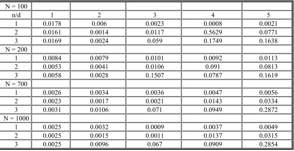
TABLE 2. Mean Squared of First-Step Forward Prediction Error of Local Polynomial Models for Different Values of Model Order (d) and Degree of Nonlinearity (n) for Mackey Glass Time Series with Different Numbers of Data.
N = 100
n/d 1 2 3 4 5
1 0.0178 0.006 0.0023 0.0008 0.0021
2 0.0161 0.0014 0.0117 0.5629 0.0771
3 0.0169 0.0024 0.059 0.1749 0.1638
N = 200
1 0.0084 0.0079 0.0101 0.0092 0.0113
2 0.0053 0.0041 0.0106 0.091 0.0813
3 0.0058 0.0028 0.1507 0.0787 0.1619
N = 700
1 0.0026 0.0034 0.0036 0.0047 0.0056
2 0.0023 0.0017 0.0021 0.0143 0.0334
3 0.0031 0.0106 0.071 0.0949 0.2872
N = 1000
1 0.0025 0.0032 0.0009 0.0037 0.0049
2 0.0025 0.0015 0.0011 0.0137 0.0315
3 0.0025 0.0096 0.067 0.0909 0.2854
as a model of white blood cell production [26].
( )
( )
(
)
(
−τ)
+ τ − α + β =
t 10 x 1
t x t x dt
t dx
(14)
Where x(t) is the value of the time series at time t. This system is chaotic for τ > 16.8. In this paper, the Mackey-Glass time series is constructed with parameter values α = 0.2, β = -0.1, τ = 30 and x0 = 1.2.
The proposed method for estimating the embedding dimension or suitable order of model based on local polynomial modeling is implemented to this time series. For this time series, the developed general program of
polynomial modeling is applied for various d and n and σ is computed for all the cases in a look up table.
Based on the discussions in Sections 2 and 3, the optimum embedding dimension is selected for this time series. The mean square of error, σ, for this chaotic system is in Table 1. According to these results, the optimum embedding dimension for this time series is estimated as 1 and 2.
TABLE 3. Mean Squared of First Step Ahead Prediction Error of Local Polynomial Models for Different Values of Model order (d) and Degree of Nonlinearity (n) for Mackey Glass Time Series with Different SNRs.
SNR = 0 dB
n/d 1 2 3 4 5 1 0.0023 0.0016 0.0029 0.0014 0.0001 2 0.0016 0.0005 0.0036 0.0145 0.0428 3 0.0134 0.0229 0.0780 0.0664 0.1226
SNR = 10 dB
1 0.0021 0.0047 0.0039 0.0019 0.0047 2 0.0044 0.0057 0.0034 0.0012 0.0035 3 0.0202 0.0049 0.0034 0.0033 0.0043
SNR = 20 dB
1 0.0114 0.0032 0.0069 0.0035 0.0075 2 0.0109 0.0041 0.0043 0.0017 0.0022 3 0.0144 0.0066 0.0052 0.0027 0.0027
SNR = 30 dB
1 0.0046 0.0096 0.0062 0.0046 0.0058 2 0.0058 0.0094 0.0035 0.0055 0.0017 3 0.0061 0.0054 0.0053 0.0017 0.0024 To show the performance of the proposed method
for embedding dimension of noisy chaotic time series, white Gaussian noise is added to this time series with different signal-to-noise ratios (SNRs). Table 3 shows the effects of noise in estimating embedding dimension for this time series. It can be seen that the performance of the proposed algorithm in estimating the minimum embedding dimension of the Mackey-Glass chaotic time series even for a noisy chaotic time series (SNR = 20 dB) is good. The “Logistic Map” is considered as the second case study in this section and the proposed method is implemented to this time series. The Logistic Map is produced by a nonlinear difference system of the form:
⎟ ⎠ ⎞ ⎜
⎝ ⎛ − =
+1 rxk 1 xk k
x (15)
Where xk is the value of the time series at time k. The time series is constructed with parameter value r = 4. Like Mackey Glass time series, the proposed method for estimating the embedding dimension or suitable order of model based on local polynomial modeling is implemented to this time series. The
mean square of error, σ, for this chaotic system has been shown in Table 4. According to these results, the optimum embedding dimension for this time series like the result of [14] is estimated 2.
At the end, the “Triangular Map” is considered and the proposed method is implemented to this time series.
The Triangular Map like Logistic Map is produced by a nonlinear difference system of the form [17]:
⎟ ⎠ ⎞ ⎜
⎝
⎛ − −
=
+1 r 1 20.5 xk k
x (16)
Where xk is the value of the time series at time k. The time series is constructed with parameter value of r = 0.91.
TABLE 4. Mean Squared of First-Step Forward Prediction Error of Local Polynomial Models for Different Values of Model Order (d) and Degree of Nonlinearity (n) for Logistic Map.
d\n 1 2 3
1 0.000074 0.000146 0.0017497
2 0.000382 0.004291 0.0001985
3 0.01006598 0.00078061 0.0001794
4 0.000428 0.0007997 0.0001294 5 0.002646 0.0002908 0.0001277
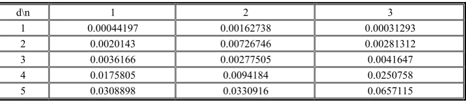
TABLE 5. Mean Squared of First-Step Forward Prediction Error of Local Polynomial Models for Different Values of Model Order (d) and Degree of Nonlinearity (n) for Triangular Map.
d\n 1 2 3
1 0.00044197 0.00162738 0.00031293
2 0.0020143 0.00726746 0.00281312
3 0.0036166 0.00277505 0.0041647
4 0.0175805 0.0094184 0.0250758
5 0.0308898 0.0330916 0.0657115
4.2. Estimation of the Embedding Dimension
for Some of the Solar Activity Indexes
Thissubsection is devoted to estimate the embedding dimension for some of the solar activity indices. These indices are, “Sun Spot Number (SSN)”,“Dst.” and “Proton Flux” indices. First of all, the “sunspot number” time series is considered.
The level of sun’s activity, defined by the occurrence of solar flares, coronal mass ejections and sunspots has quasi periodic variations with a period of about eleven years. Each eleven-year solar cycle starts with a period of quiescence called solar minimum and gradually turns into a period of activity called solar maximum [24,25].
The sunspot number is a good measure of solar activity and is computed according to the Wolf formulation:
R = k (10g + s) (17)
Where g is the number of sunspot groups, s is the
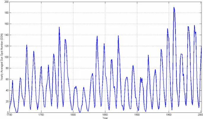
total number of spots in all groups and k is a variable scaling factor which is related to the conditions of observation. The monthly and yearly averaged number of sunspots is accessible through several web sites from the sunspot Index Data Center in Belgium or US National Oceanic and Atmospheric Administration. In this paper yearly averaged number of sunspots is used for estimating embedding dimension of this time series. Figure 2 shows this time series.
The proposed method for estimating the embedding dimension is implemented to this solar activity index. For this time series, for various d and n, σ is computed. Based on the discussions in Sections 2 and 3, the optimum embedding dimension is selected for this time series. The mean square of error, σ, for this chaotic system has been shown in Table 6. According to these results, the optimum embedding dimension for this time series is estimated as 2 and 4.
Figure 2. Yearly averaged number of sun spot during 1700 to 2001.
TABLE 6. Mean Squared of First-Step Ahead Prediction Error of Local Polynomial Models for Different Values of Model Order (d) and Degree of Nonlinearity (n) for Sun Spot Number.
d\n 1 2 3
1 0.0055 0.0050 0.0080
2 0.0036 0.0033 0.0099
3 0.0095 0.0119 0.0089
4 0.0118 0.0107 0.0038
5 0.0140 0.0074 0.0053
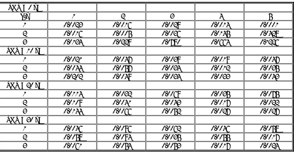
TABLE 7. Mean Squared of First-Step Ahead Prediction Error of Local Polynomial Models for Different Values of Model Order (d) and Degree of Nonlinearity (n) for Sunspot Number Time Series with Different Numbers of Data.
N = 100
n/d 1 2 3 4 5
1 0.0368 0.0026 0.0086 0.0125 0.0172 2 0.0344 0.0114 0.0107 0.0053 0.01 3 0.0346 0.0029 0.012 0.0012 0.0026 N = 200
1 0.0261 0.0044 0.0115 0.0066 0.0083 2 0.0247 0.003 0.0075 0.0099 0.0095 3 0.0236 0.0085 0.0061 0.0044 0.0061 N = 301
Figure 3. The performance of the proposed method in one-step ahead prediction og sunspot number time series:
(Upper) the predicted time series vs. the actual value for test set; (Lower) the prediction error.
series. It can be seen that the performance of the proposed algorithm in estimating the minimum embedding dimension of the sunspot number as a natural noisy chaotic time series even with a few numbers of data is good.
To check the performance of the model for the reconstructed SSN dynamic, this model is used for one-step forward prediction of sunspot number time series. The estimated embedding dimension and degree of nonlinearity is used for this model. 201 data from 1700 to 1900 is used for training and remaining 100 data from 1901 to 2001 is used for testing. Figure 3 shows the performance of this method in one-step forward prediction of sunspot number time series. Although this method is not proposed for prediction, but the performance of the trained model is good enough.
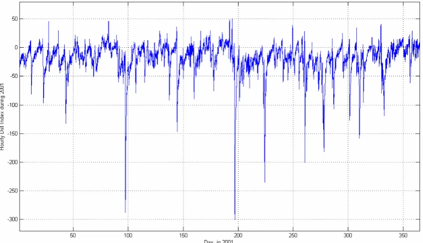
The Dst. is considered as the next solar activity indices and the proposed method is implemented to this time series. Like SSN, the hourly and daily averaged value of Dst. is accessible through
several web sites from the sunspot Index Data Center in Belgium or US National Oceanic and Atmospheric Administration. In this paper, the hourly value of Dst. in 2001 is considered to be used for estimating the embedding dimension for this index. Figure 4 shows this index during 2001. The proposed method for estimating the embedding dimension is implemented to this index. The mean square of error, σ, for this chaotic system has been shown in Table 8. According to these results, the optimum embedding dimension for this time series is estimated as 1 and 5.
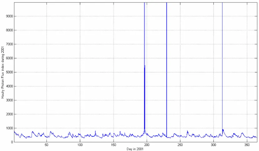
At the end, the “proton flux” is considered and the proposed method is implemented to this solar activity indices. To estimate the embedding dimension for this time series, the hourly value of “proton flux” is considered for estimation. Figure 5 shows “proton flux” during 2001.
Figure 4. Hourly Dst. index during 2001.
TABLE 8. Mean Squared of First Step Ahead Prediction Error of Local Polynomial Models for Different Values of Model Order (d) and Degree of Nonlinearity (n) for Dst.
d\n 1 2 3
1 0.0033 0.0432 0.0283
2 0.0160 0.0228 0.0571
3 0.0010 0.0161 0.0738
4 0.0009 0.0014 0.0363
5 0.0006 0.0012 0.0581
for this time series is equal to 2. The adaptive method for calculating the Lyapunov exponents is implanted in this time series and like two other time series it is shown that the first and the biggest Lyapunov exponents has positive trend and like other indexes it is not possible to predict this index after a while. Figure 5 shows the trend of the Lyapunov exponents for this chaotic time series. According to these results, the optimum
embedding dimension for each chaotic system is estimated in Table 10.
5. DISCUSSION AND CONCLUSIONS
Figure 5. Hourly proton flux during 2001.
TABLE 9. Mean Squared of First Step Ahead Prediction Error of Local Polynomial Models for Different Values of Model Order (d) and Degree of Nonlinearity (n) for Proton Flux index.
d\n 1 2 3
1 0.0028 0.0077 0.0208
2 0.0034 0.0012 0.0106
3 0.0032 0.0026 0.0032
4 0.0015 0.0004 0.0012
5 0.0025 0.0005 0.0014
TABLE 10. The Estimated Optimum Embedding Dimension d for Each Chaotic System.
Chaotic Systems d
Mackey Glass Time Series 1-2
Logistic Map 1
Triangular Map 1
Sun Spot Number (SSN) index. 1-4
Dst. Index 2-5
polynomial modeling for solar activity dynamics as well-known natural chaotic time series is proposed. After fitting a general polynomial autoregressive model to the given time series, a canonical state space realization of the system is obtained. Then, the normalized one-step forward prediction error is measured to estimate the minimum embedding dimension. Moreover, the resulting local model can be used for prediction and Lyapunov exponents’ estimation as well. Finally, the simulation results of applying the method to some well-known chaotic systems and solar activity indices which their optimal value for embedding dimension is the purpose of this paper provided that these results depict the great performance of this method in estimating the embedding dimension of such chaotic systems.
6. ACKNOWLEDGEMENTS
The authors wish to thank the reviewers of “International Journal of Engineering” for their helpful suggestions and bringing further references to the attention of the authors.
7. REFERENCES
1. Mirmomeni, M., Lucas, C. and Kamaliha, E., “Predicting Chaotic Time Series Using Co-Evolution of Models and Tests”, 26th Int. Symp. on Forecasting, Santander, Spain, (June 2006), 105-110.
2. Packard, N. H., Crutchfield, J. P., Farmer, J. D. and Shaw, R. S., “Geometry from a Time Series”, Phys. Rev. Lett., Vol. 45, (1980), 712-716.
3. Takens, F., “Detecting Strange Attractors in Turbulence”, Lecture Notes in Mathematics, Eds. Rand, D. A. Young, L. S., Springer, Berlin, Germany, Vol. 898, (1981), 366-381.
4. Sauer, T., Yorke, J. A. and Casdagli, M., “Embedology”, J. Stat. Phys., Vol. 65, No. 3-4, (1991), 579-616.
5. Kennel, M. B., Brown, R. and Abarbanel, H. D. I., “Determining Embedding Dimension for Phase Space Reconstruction Using a Geometrical Construction”, Phys. Rev. A., Vol. 45, (1992), 3403-3411.
6. Ataei, M., Khaki-Sedigh, A., Lohmann, B. and Lucas, C., “Determining Embedding Dimension from Output Time Series of Dynamical Systems-Scalar and Multiple Output Cases”, Proc. of the 2nd Int. Conf. on System Identification and Control Problems, Moscow, Russia,
(2003), 1004-1013.
7. Cao, L., “Practical Method for Determining the Minimum Embedding Dimension of a Scalar Time Series”, Physica D., Vol. 110, (1997), 43-50.
8. Broomhead, D. S. and King, G. P., “Extracting Qualitative Dynamics from Experimental Data”, Physica D., Vol. 20, (1986), 217-236.
9. Ataei, M., Khaki-Sedigh, A., Lohmann, B. and Lucas, C., “Determining Embedding Dimension Using Multiple Time Series Based on Singular Value Decomposition”, Proc. of the 4th Int. Symp. on Mathematical Modeling, Vienna, Austria, (2003), 190-196.
10. Paluš, M. and Dvoŕăk, I., “Singular-Value Decomposition in Attractor Reconstruction: Pitfalls and Precautions”, Physica D., Vol. 55, (1992), 221-234. 11. Mess, A. I., Rapp, P. E. and Jennings, L. S.,
“Singular-Value Decomposition and Embedding Dimension”, Phys. Rev. A., Vol. 36,(1987), 340-346.
12. Fraser, M., “Reconstructing Attractors from Scalar Time Series: A Comparison of Singular System and Redundancy Criteria”, Physica D., Vol. 34, (1989), 391-404.
13. Bian, C. H. and Ning, X. B., “Determining the Minimum Embedding Dimension of Nonlinear Time Series Based on Prediction Method”, Chinese Physics, Vol. 13, No 5, (2004), 633-936.
14. Meng, Q. F., Peng, Y. H. and Xue, P. J., “A new Method of Determining the Optimal Embedding Dimension Based on Nonlinear Prediction”, Chinese Physics, Vol. 16, No. 5, (2007), 1252-1257.
15. Grassberger, P. and Procaccia, I., “Measuring the Strangeness of Strange Atractors”, Physica D., Vol. 9, (1983), 189-208.
16. Ataei, M., Khaki-Sedigh, A., Lohmann, B. and Lucas, C., “Model Based Method for Determining the Minimum Embedding Dimension from Chaotic Time Series Univarite and Multivariate Cases”, Nonlinear Phenomena in Complex Systems, Vol. 6, No. 4, (2003), 842-851.
17. Ataei, M., Khaki-Sedigh, A., Lohmann, B. and Lucas, C., “Model Based Method for Estimating an Attractor Dimension from Uni/Multivariate Chaotic Time Series with Application to Bremen Climatic Dynamics”, Chaos, Solitons and Fractals, Vol. 19, (2004), 1131-1139.
18. Landau, D., Lozano, R. and M’Saad, M., “Adaptive Control”, Springer-Verlag, Berlin, (1989).
19. Isermann, R., “Adaptive Control Systems”, Prentice-Hall, Inc., Englewood Cliffs, New Jersey, U.S.A., (1991).
20. Ljung, L., “System Identification: Theory for the User”, Prentice-Hall, Inc., Englewood Cliffs, New Jersey, U.S.A., (1998).
21. Nelles, O., “Nonlinear System Identification”, Springer Verlag, Berlin, (2001).
22. Casdagli, M., “Nonlinear Prediction of Chaotic Time Series”, Physica D., Vol. 35, (1989), 335-356.
Prediction”, Journal of Neural Computing and Applications, Vol. 16, No. 4-5, (2007), 383-393.
24. Mirmomeni, M., Shafiee, M., Lucas, C. and Araabi, B. N., “Introducing a New Learning Method for Fuzzy Descriptor Systems with the Aid of Spectral Analysis to Forecast Solar Activity”, Journal of Atmospheric and Solar-Terrestrial Physics, Vol. 68, (2006), 2061-2074.
25. Mirmomeni, M., Lucas, C., Araabi, B. N. and Shafiee, M., “Forecasting Sunspot Numbers with the Aid of Fuzzy Descriptor Models”, Space Weather, Journal of Research and Applications, Doi: 10.1029/2006SW000289, (2007). 26. Mackey, M. and Glass, L., “Oscillation and Chaos in