Please cite this article as: A. Karami-Mollaee,Adaptive Fuzzy Dynamic Sliding Mode Control of Nonlinear Systems, International Journal of Engineering (IJE), TRANSACTIONS B: Applications Vol. 29, No. 8, (August 2016) 1075-1086
International Journal of Engineering
J o u r n a l H o m e p a g e : w w w . i j e . i rAdaptive Fuzzy Dynamic Sliding Mode Control of Nonlinear Systems
A. Karami-Mollaee
Department of Electrical and Robotic Engineering, University of Shahrood, Shahrood, Iran
P A P E R I N F O
Paper history: Received 19 October 2015
Received in revised form 29 May 2016 Accepted 02 June 2016
Keywords: Fuzzy Control
Dynamic Sliding Mode Control Chattering
Adaptive Control Chaotic System
A B S T R A C T
Two phenomena can produce chattering: switching of input control signal and the large amplitude of this switching (switching gain). To remove the switching of input control signal, dynamic sliding mode control (DSMC) is used. In DSMC switching is removed due to the integrator which is placed before the plant. However, in DSMC the augmented system (system plus the integrator) is one dimension bigger than the actual system and then, the plant model should be completely known. To overcome this difficulty, a fuzzy system is employed to identify the unknown nonlinear function of the plant model and then, a robust adaptive law is developed to train the parameters of this fuzzy system. The other problem is that the switching gain may be chosen unnecessary large to cope on the unknown uncertainty. To solve this problem, another fuzzy system is proposed which does not need the upper bound of the uncertainty. Moreover, to have a suitable small enough switching gain an adaptive procedure is applied to increase and decrease the switching gain according to the system circumstances. Then, chattering is removed using the DSMC with a small adaptive switching gain (ASG). As a case study, nonlinear chaotic Duffing-Holmes system is selected.
doi: 10.5829/idosi.ije.2016.29.08b.07
1. INTRODUCTION1
1. 1. Sliding Mode Control (SMC) It has been shown that the SMC, because of its invariance property, is a powerful tool in facing structured or unstructured uncertainties and disturbances that always produce difficulties in the realization of designed controller for real systems [1-3]. Note that invariance is stronger than robustness [3].
The invariance property is the motivation of researchers in use of SMC for various applications [4-7] especially is precise systems [8]. The greatest shortcoming of SMC is chattering, the high (but finite) frequency oscillations with small amplitude that produce heat losses in electrical power circuits and wear mechanical parts [3]. Chattering is often due to the excitation of high frequency un-modeled (ignored) dynamics (sensors, actuators and plant) [9]. Excitation of these dynamics is due to two causes: high controller gain and high frequency switching of input control signal [9].
1*Corresponding Author’s Email: [email protected] (A. Karami-Mollaee)
switching. For example, it has been shown [16] that in HOSMC chattering may happen in some methods such as power-fractional algorithm and super-twisting algorithm. Both of these algorithms utilize a continuous nonlinear function with infinite gain. In DSMC an integrator (or any other strictly low-pass filter) is placed before the input control signal of the plant [17]. Then, switching is removed from the input control signal since the integrator filters the high frequency switching which is, due to the use of SMC [17]. However, in DSMC the augmented system is one dimension bigger than the actual system and then the plant model should be completely known when one needs to use SMC to control the augmented system states [17].
1. 3. Fuzzy Systems In the past decades, fuzzy logic is used in the structure of controllers in nonlinear systems [18] and researchers have proposed various fuzzy SMC (FSMC) methods (see [18] and references therein). Generally, these methods can be classified into two categories: direct and indirect approaches [18]. In direct approaches, SMC is implemented by a fuzzy system. But, in indirect approaches, fuzzy system is used to meet a secondary goal in SMC.
1. 4. The Proposed Approach SMC consists of three phases: reaching phase (the time needed for hitting to the sliding surface), sliding phase (sliding on a stable manifold) and steady state phase [1]. To preserve the invariance property during the sliding and steady state phases and guarantee reaching to the sliding surface in finite time, one should use the reaching law [9]:
) (s sign
s where, is a positive large enough constant. It is known that use of this sign function causes, high frequency switching with amplitude , called the switching gain [9]. The switching gain should be greater than the upper bound of the uncertainty [1, 3, 9]. But, in practical systems this bound is usually unknown. This leads to a large conservative value of and may cause an unsuitable control effort. Therefore, from an engineering point of view, a controller that can be auto-adjusted with ASG seems interesting. Therefore, chattering can be suppressed by [9]:
1. Removing the effect of high frequency switching of input control signal.
2. Reducing the amplitude of the switching, i.e., reducing the switching gain.
In this paper a method is presented, having the above two characteristics, by employing ASG and DSMC. Therefore, the proposed method will alleviate the two reasons that can excite un-modeled dynamics. Two fuzzy networks are implemented. The first indirect fuzzy system is used to overcome the drawback of DSMC and is employed to identify the plant model. The second direct fuzzy system is used as a controller which does not need the upper bound of the uncertainty. To
guarantee the robustness of these fuzzy networks (fuzzy identification network and fuzzy controller network), a new robust adaptive law is developed for each network. Finally, an adaptive procedure is proposed which results the suitable small enough switching gain. According to this adaptive procedure, the gain of the switching increases or decreases based on the system conditions. Then, chattering is removed completely using the DSMC with a small ASG.
1. 5. Paper Organization The remainder of this paper is organized as follows: in section 2 we provide the preliminary background about the problem. In section 3 the fuzzy identification method is proposed. Section 4 is devoted to design adaptive fuzzy DSMC methodology. In section 5 we have a brief comparison. Then, in section 6 we discuss simulation results to verify theoretical concepts presented in previous sections. The conclusion is given in section 7. For simplicity of reading the paper, the proof of theorems and lemma is in a separate section as an appendix (section 8).
2. PROBLEM FORMULATION
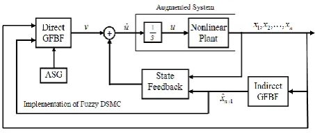
The proposed approach is depicted in Figure 1 and we will describe each block diagram in the next sections. Consider the following single input nonlinear system:
) , (
1 , , 2 , 1 : 1
u X f x
n i
x x
n i i
(1)
with input u and accessible states T
n x x x
X[1, 2, ] . Note that the function f(X,u) is unknown. The goal is to have the states of this system, i.e. vector X, track the states of the following stable linear system, i.e. variables
n i
yi: 1,2,, , which is used as a reference model.
d n
i i i n
i i
u y d y
n i
y y
1
1: 1,2, , 1
(2)
and di(t):i1,2,,n can be time varying coefficients. Equation (1) can be written as follows:
) , (X u f B X A
X (3)
Matrixes A and B are with appropriate dimensions.
1 0 0 0
,
0 0 0 0
1 0 0 0
0 1 0 0
0 0 1 0
B
A (4)
We can write:
) , ( )
(A A X Bf X u X
A
X s s (5)
or:
) , (X u g B X A
X s (6)
where:
n
i i ix
a u X f u X g
1
) , ( ) ,
( (7)
and:
n
n s
a a a a A
1 2
1
1 0 0 0
0 1
0 0
0 0
1 0
(8)
Assume that ai are such that As is stable, i.e., for any symmetric positive definite matrix Q, there exists a symmetric positive definite matrix P satisfying the following Lyapunov equation:
Q A P P
ATs s (9)
3. IDENTIFACATION ALGORITHMS
According to the fuzzy theorems, Gaussian fuzzy basis functions (GFBF) can approximate any real continuous function on a compact set with any arbitrary accuracy. This means that the GFBF has universal approximation property [19]. In order to estimate the nonlinear function
g
(
X
,
u
)
, a singleton fuzzifier with product inference engine and a defuzzifier as weight sum of each output rule is used”) , ( ˆ
ˆ w X u
g T
(10)where wˆm is the weight vector estimate of rules, and (.):n1m is the Gaussian membership function (GMF) vector. Then, the fuzzy model of Equation (6) can be written as:
) , ( ˆ ˆ
ˆ A X Bw Xu
X s T (11)
where Xˆ[xˆ1,xˆ2,xˆn]T is the identified model state vector. Due to the approximation capability of the GFBF, there exists an ideal weight vector
w
with arbitrary large enough dimension m such that the system (6) can be written as follows:X T
sX Bw X u B A
X ( , ) (12)
where X is an arbitrary small reconstruction error. We also make the following two assumptions. Where, are common in the control systems literature and are due to universal approximation property of the GFBF.
Assumption 1: The GFBF reconstruction error is bounded by B, i.e. X B.
Assumption 2: The ideal weight is bounded by a known positive value Bw such that w Bw.
Now, the following estimator is proposed:
) ˆ ( ) , ( ˆ ˆ
ˆ A X Bw X u k X X
X s T x (13)
By subtracting (13) from (12), we obtain:
X k B u X w B X A
X s T X x
~ )
, ( ~ ~
~ (14)
where X~(t)X(t)Xˆ(t) and w~wwˆ are the state and parameter estimation errors.
Theorem 1: Given the assumptions 1 and 2 for the system (12) and the estimator (13), and using the following weight adaptive law:
w X k k X B P u X k
w w T e w ˆ
~ 4 ~ ) ( ) , (
ˆ
(15)
Then, estimation error X~(t) converges to zero if
x
k .kw and ke are arbitrary positive scalar constants and min(Q) and min(P) are the smallest eigenvalues of positive definite matrices Q and P, which satisfy Lyapunov Equation (9) and max(P) is the largest eigenvalue of
P
.Proof: In appendix, from Equations (A.1) to (A.10). Remark 1: The result of this theorem can be written as:
0 ~ lim
X
t
kx (16)
4. CONTROLLER DESIGN
A. State feedback
According to Equations (7) and (10) we can write:
X CA u X w u X
where,C[0,0,0,1]n. To apply the DSMC to system (1), we define the following augmented system:
u x x x n i x x u X f x n n n i i n 1 1 1 1 ˆ ˆ 1 , , 2 , 1 : ) , ( ˆ ˆ (18)
where xˆn1 is the fuzzy identification of unknown variable xn1 and:
u w u X X CA X X w w u x
X n T T s T
( , 1, ) ˆ ˆ , ( , ) ˆ (19)
Now, we define the following variables:
Y X e e e E y x e n i y x e x x x x X y y y Y t d t d t d D a T n n n n i i i T n n a T n n ] , , , [ ˆ , , 2 , 1 : ] ˆ , , , , [ ] , , , [ )] ( , ), ( ), ( , 0 [ 1 2 1 1 1 1 1 2 1 1 2 1 2 1 (20)
Then, augmented reference system can be written as follows: d n i i d n i i i n u DY y n i y y u y d y
1 1 1 1 , , 2 , 1 : (21)Then, we have:
) (
) (
ˆ 1 1
1 v DX u u u u v DE u u v v DX DX u DY u u DY u y x e a d a a d d n n n (22)
We define the following linear state feedback.
v DX
u a (23)
and the following variable:
d
u u u
W() (24)
We obtain:
W v DE
en1 (25)
Such that, v is the new input control signal to be calculated via SMC and W(X,xn1,u,u) is a matched uncertainty. The matched uncertainty can be cancelled out directly by the input [8].
Remark 2: Variable W is considered as uncertainty due to its dependency to unknown variable xn1.
The control problem now is finding a suitable input control signal v(t) such that the states of system (18),
a
X , track the states of system (21), Y, or equivalently the error dynamics E in (25) converge to zero in finite time.
B. Fuzzy adaptive controller with ASG
Now, we define the following sliding surface.
dt e e e e t e t
s n
t n n n n 0 1 1 2 2 11
1() ( )
)
( (26)
From the universal approximation capability of GFBF, there exist ,
, and c such that: ( (), , , ) )
(t v st c
v f (27)
where, is the approximation error and vf is a fuzzy system in the following form with input s(t).
) ) ( exp( ) , , ( )] , , ( , ), , , ( ), , , ( [ ) , , ( ] , , , [ ) , , ( ) , , ( 2 2 2 2 2 1 1 1 2 1 1 i i i i i T M M M T M T M i i i i i f c s c s c s c s c s c s c s c s v
(28)In this stage, we propose the following control law.
)) ( ( ) ˆ , ˆ , ˆ ), ( ( ˆ )
(t v st c v st
v f c (29)
where vˆf is the approximation of vf and ˆ ,
ˆ, and cˆ are estimates of the desired parameters ,
, and c. Moreover, vc is the compensation controller to compensate the approximation error . Applying (29), Equation (25) becomes:W v v DE
en1 ˆf c (30)
Consequently: c f n n n n
n e e e e v v v
e t
s()11 1 2211 ˆ (31)
Defining, v~f vvˆf we have:
ˆ ˆ ˆ
~ T T
f f
f v v
v (32)
Now define ~ˆ and ~ˆ then:
~ ~ ˆ ~ ~ ˆ ˆ ˆ ) ~ ˆ ( ) ~ ˆ ( ~ T T T T T f v (33)
If the vector of GMF is linearized using Taylor series expansion, ~ can be written as:
T O H B c
At~ t~ . .
~
(34) ˆ 2 1 ˆ 2 1 , , , , , , M t c c M t B c c c A (35) T M i i i i T M i i i i c c c c , , , , , , 2 1 2 1 (36)
Substituting (34) into (33) leads to:
ˆ ~ ~ ˆ ~ ˆ ~ ~ ˆ ~ ) . . ~ ~ ( ˆ ~ T t T t T T T t t T f B c A T O H B c A v (37)
Now, we use Equations (31) and (37):
c T t T t T v B c A t
s()ˆ ~ˆ ~~ ˆ (38)
Such that ˆTH.O.T~T~ is the uncertain term and is assumed to be bounded by a constant bound, i.e.
. We assume that this bound is unknown and use an estimate of it denoted by ˆ. Here, we propose a method which can decrease or increase the switching gain ˆ according to the system conditions. In the proposed approach, ˆ(t) is defined as follows:
) 0 ( ˆ ˆ , ) ) ( ( ˆ ) ( ˆ 0 0 1
0
t
t s d (39)or:
0 1( (ˆ)),ˆ(0) ˆ
ˆ
s (40)
and:
(ˆ ) 1
02 ) ˆ
( 1 0
sign (41)
Constants q20, 10 and 0 0 are design parameters and ˆ0 ˆ(0) is the bounded initial value of ˆ(t). Note that we can select ˆ0 arbitrary.
Lemma 1: If the following condition is satisfied:
0 0
ˆ
(42)
Then, the ASG of Equations (40) and (41) guarantee that:
0 : )
(
ˆt 0 t
(43)
Proof: In appendix, form Equations (B.1) to (B.9). Theorem 2: Consider the error dynamics (30) with the input control signal of (29). Then, the error trajectory converges to zero if the following adaptation laws are incorporated.
) ( ˆ 0 1 ) ˆ ( 2 ) ˆ ( ˆ ) 0 ( ˆ )), ˆ ( ( ˆ ˆ ˆ ˆ ˆ ˆ ˆ 0 1 0 0 1 4 3 2 s sign v sign s sB sA c s c T t T t (44)Proof: In appendix, from Equations (C.1) to (C.7).
5. ADVANTAGES AND COMPARISON
The other choice of ASG is as follows [20]:
0 1 ,ˆ(0) ˆ
ˆ
s (45)
Despite the fact that this ASG shows that the estimated switching gain ˆ is increased until the error trajectory is driven into sliding mode, this ASG has three severe practical disadvantages:
1. In case of a large initial distance from the sliding surface, the estimated switching gain will increase quickly due to this error and not because of perturbation. This may result in a switching gain which is significantly larger than necessary.
2. Noise on the measurements will prevent s to ever become exactly zero, so increase of the adaptive estimated switching gain will continue. This causes instability of the closed loop system. The rate of increase depends on the value of 1.
3. The adaptation law can only increase the estimated switching gain but never decrease it. Thus if the circumstances change such that a smaller switching gain is permitted, the adaptation law is not able to adapt to these new circumstances.
But, the proposed approach in Equations (40) and (41) has the following advantages:
1. In the case of a large initial distance from the sliding surface, the estimated switching gain will increase quickly, resulting the distance to shrink. Once this distance is smaller than 1, this gain will decrease again.
2. Noise on the measurements does not disturb the adaptation procedure if the constant 1 is not chosen very small.
3. The ASG law can increase ˆ(t) again according to lemma 1. Moreover, ˆ(t) will not converge to zero.
6. SIMULATION RESULTS
) ( ) ( ) cos( ) ( ) ( ) ( ) (
) ( ) (
1 3
1 2 2 1 1 2
2 1
t d t u t q t x t x p t x p t x
t x t x
(46)
To ensure the existing of chaos in the absence of control, the parameters p1, p2, q and 1 are chosen as p11, p20.25, q0.3 and 11 with the
initial condition of T T
x x
X(0)[1(0), 2(0)] [1,2.5] . Then, we have:
) ( ) ( ) cos(
) ( ) ( ) ( ) , , (
1
3 1 2 2 1 1 2
1 3
t d t u t q
t x t x p t x p u x x f x
(47)
For the indirect fuzzy system we choose a GMF vector with three inputs (x1,x2,u) and nine rules as follow:
9 , , 2 , 1 : 5 ) 5 ( exp
) , , (
2 2 2 2 1 2 1
i i u x x u x x
i
(48)
The output of defuzzifier is fˆ(x1,x2,u). The indirect fuzzy network tuning parameters are chosen as kw 5,
70
x
k and ke30 . Other parameters are chosen as:
8 9
1 0 , 500 400
300 400
s A
P (49)
The initial conditions of the weight vector are chosen as
Tw(0) 0,0,,0 . Notice that, these initial conditions can be chosen arbitrary. The objective is to make the states of system (46) track the states of the following linear system:
d
u y y y
y y
2 1 2
2 1
3 5
(50)
Moreover, ud is a periodic step signal and ]
3 , 5 , 0 [
D . All the initial conditions of the
parameters , c,
are set to be zero and ˆ0 0.05 and also we choose M 9. Moreover:5 . 0 , 5 , 10 , 5 .
0 2 3 4
1
(51)
In both simulations we applied an external load disturbance d(t)1 at t10s and also:
2 . 0 , 15 .
0 1
0
(52)
The simulations are done by MATLAB with sample time of 0.001. The procedure for calculating u is as follows:
1. Define and calculate (X,u) as Equation (48). 2. Calculate weight vector wˆ from Equation (15). 3. Calculate fˆ(X,u) from Equation (17).
4. Calculate sliding surface using Equation (26). 5. Calculate parameters of Equation (44). 6. Calculate v via Equation (29). 7. Calculate u using Equation (23).
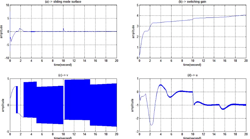
8. Calculate u by numerical integrating of u. Figures (2), (3) and (4) show the simulation results. From Figure (4.b) we can see that the switching gain increases at first to force the error trajectories toward the sliding surface but it decreases when the trajectories reach near the surface while, the input control of system is without switching (Figure (4.d)). From Figure (4.b)
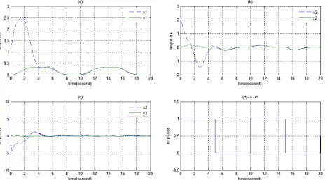
Figure 3. Reference signal tracking of augmented system: (a) first state, (b) second state, (c) third state and (d) input control signal of reference system.
Figure 4. (a) Sliding surface, (b) switching gain, (c) input control signal of state feedback and (d) input control signal of system.
we can see that at t10s the switching gain increases to overcome on the disturbance and then starts to decrease again.
To show the effectiveness of the proposed method the simulation has been done using Equation (45). Figures
(5), (6) and (7) show the simulation results. From Figure (7.b) we can see increase of switching gain which leads to unstability. Moreover, the switching gain increases (Figure (7.d)). From Figure (7.b) we can see that at
s
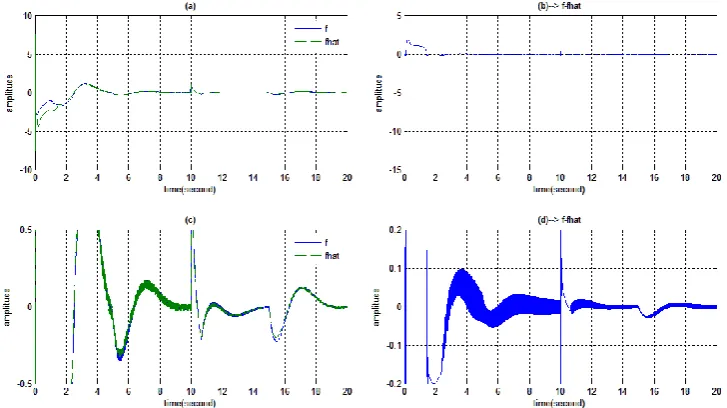
Figure 5. (a) and (c) f and its estimation fˆ (output of the indirect fuzzy system), (b) and (d) error between the fˆ and its actual value f.
Figure 7. (a) Sliding surface, (b) switching gain, (c) input control signal of state feedback and (d) input control signal of system.
7. Conclusion
In this paper, a new method for designing DSMC based on variable structure control technique is proposed for
nonlinear systems. Two fuzzy networks are
implemented. To solve the problem of DSMC an indirect fuzzy system is employed to identify the unknown nonlinear function of the plant model and then a robust adaptive law is developed to train the parameters of the fuzzy network. The second direct fuzzy system is used as a controller; use of an upper bound for uncertainty is not necessary in design of the controller. Therefore, proposed approach will be applicable to practical systems where this bound may not be known. Then, an adaptive switching gain is used to guarantee increase and decrease of the switching gain according to the system conditions. Then, chattering is removed due to the implementation of DSMC via adaptive switching gain. The proposed method also preserves the main property of SMC such as invariance. The proposed method is applied for synchronization of a chaotic system. Simulation results show the effectiveness of this method.
9. REFERENCES
1. Slotine, J.-J.E. and Li, W., "Applied nonlinear control, prentice-Hall Englewood Cliffs, NJ, Vol. 199, (1991(.
2. Young, K.D., Utkin, V.I. and Ozguner, U., "A control engineer's guide to sliding mode control", IEEE transactions on control systems technology, Vol. 7, No. 3, (1999), 328-342.
3. Perruquetti, W. and Barbot, J.-P., "Sliding mode control in engineering, CRC Press, (2002(.
4. Sun, T., Pei, H., Pan, Y., Zhou, H. and Zhang, C., "Neural network-based sliding mode adaptive control for robot manipulators", Neurocomputing, Vol. 74, No. 14, (2011), 2377-2384.
5. Zhang, M.-j. and Chu, Z.-z., "Adaptive sliding mode control based on local recurrent neural networks for underwater robot",
Ocean Engineering, Vol. 45, (2012), 56-62.
6. Zou, Y. and Lei, X., "A compound control method based on the adaptive neural network and sliding mode control for inertial stable platform", Neurocomputing, Vol. 155, (2015), 286-294. 7. Mefoued, S., "A second order sliding mode control and a neural
network to drive a knee joint actuated orthosis",
Neurocomputing, Vol. 155, (2015), 71-79.
8. Kim, H.M., Park, S.H. and Han, S.I., "Precise friction control for the nonlinear friction system using the friction state observer and sliding mode control with recurrent fuzzy neural networks",
Mechatronics, Vol. 19, No. 6, (2009), 805-815.
9. Lee, H. and Utkin, V.I., "Chattering suppression methods in sliding mode control systems", Annual reviews in control, Vol. 31, No. 2, (2007), 179-188.
10. Park, S. and Rahmdel, S., "A new fuzzy sliding mode controller with auto-adjustable saturation boundary layers implemented on vehicle suspension", International Journal of Engineering-Transactions C: Aspects, Vol. 26, No. 12, (2013), 1401. 11. Chen, M.-S., Hwang, Y.-R .and Tomizuka, M., "A
state-dependent boundary layer design for sliding mode control",
IEEE transactions on automatic control, Vol. 47, No. 10, (2002), 1677-1681.
12. Levant, A., "Sliding order and sliding accuracy in sliding mode control", International journal of control, Vol. 58, No. 6, (1993), 1247-1263.
13. Bartolini, G., Ferrara, A. and Usani, E., "Chattering avoidance by second-order sliding mode control", IEEE transactions on automatic control, Vol. 43, No. 2, (1998), 241-246.
14. Oh, S. and Khalil, H.K., "Nonlinear output-feedback tracking using high-gain observer and variable structure control",
15. Levant, A., "Robust exact differentiation via sliding mode technique", Automatica, Vol. 34, No. 3, (1998), 379-384. 16. Boiko, I., Fridman, L. and Iriarte, R., "Analysis of chattering in
continuous sliding mode control", in Proceedings of the 2005, American Control Conference, 2005., IEEE., (2005), 2439-2444. 17. Chen, M.-S., Chen, C .- H. and Yang, F.-Y., "An
ltr-observer-based dynamic sliding mode control for chattering reduction",
Automatica, Vol. 43, No. 6, (2007), 1111-1116.
18. Kaynak, O., Erbatur, K. and Ertugnrl, M., "The fusion of computationally intelligent methodologies and sliding-mode control-a survey", IEEE Transactions on Industrial Electronics, Vol. 48, No. 1, (2001), 4-17.
19. Tanaka, K. and Wang, H.O., "Fuzzy control systems design and analysis: A linear matrix inequality approach, John Wiley & Sons, (2004).
20. Lin, C.-M. and Hsu, C.-F., "Adaptive fuzzy sliding-mode control for induction servomotor systems", IEEE Transactions on Energy Conversion, Vol. 19, No. 2, (2004), 362-368.
21. Sifakis, M. and Elliott, S., "Strategies for the control of chaos in a duffing–holmes oscillator", Mechanical Systems and Signal Processing, Vol. 14, No. 6, (2000), 987-1002.
22. Li, W., Lan, T. and Lin, W., "Adaptive tracking control of duffing-holmes chaotic systems with uncertainty", in Computer Science and Education (ICCSE), 2015 0th International Conference on, IEEE., (2010), 1193-1197.
8. APPENDIX: PROOF OF THEOREMS AND LEMMAS
Proof of Theorem 1: Consider the following Lyapunov function: w w k X P X t V T w
T ~ ~
2 1 ~ ~ 2 1 )
( (A.1)
Taking the derivative of V(t) yields:
w w k X P X X P X t V T w T
T
~ ~ 1 ~ ~
2 1 ~ ~ 2 1 )
( (A.2)
Substituting Equations (9) and (14) in the above equation gives: X B P u X w k w X X k P X B P X X Q X t V T w T x T X T T ~ ) ( ) , ( ~ 1 ~ ) ˆ ( ~ ~ ~ ~ 2 1 ) ( (A.3)
since w~ wˆ, using the tuning law (15) in the above equation gives: w w X k X P X k B P X X Q X t
V ~T ~ ~T X x~T ~ 4 e ~~Tˆ 2
1 )
(
(A.4)
Considering the properties of positive definite matrixes Q and P, and using wˆ ww~, the above equation yields:
P B k w B w
XX P k Q t V w e x ~ ) ~ ~ ( 4 ) ( ~ ) ( ) ( ) ( 2 max 2 min min 2 1 (A.5)
Now, we define BX~ as follows:
) ( ) ( 2 1 ) ( min min 2 max ~ P k Q B k B P B x w e X (A.6) Therefore:
X B w k B X X P k Q t V w e X x ~ ~ 4 ~ ~ ) ( ) ( ) ( 2 2 1 ~ min min 2 1 (A.7) or:
Q kx P
X
X BX
t
V min min ~
2
1 ~ ~
) ( ) ( ) ( (A.8)
Take
X
x P X X B
k Q
t min min ~
2
1 ~ ~
) ( ) ( ) (
and
suppose X~ BX~ then, one can write V(t)0. Integration from zero to t yields:
) 0 ( ) ( ) ( ) ( 0 0
0 d d V t V
t t
(A.9)when t, the above integral exists and is less than or equal to V(0). Since V(0) is positive and finite, according to the Barbalat’s lemma [1] we will have:
( ) ( )
~
~
0lim ) (
lim min min ~
2
1
x X
t
t t Q k P X X B (A.10)
and note that
min( ) min( )
21
P k
Q x
is greater than
zero. Then, (A.10) implies that
X t
B
X~ ~
lim
whose
result is decreasing X~ until it becomes less than BX~. This guarantees that BX~ is the upper bound of X~ and it is clear that lim ~0
X
kx B
. Then, X~ or X~ will
converge to zero if kx.
Proof of Lemma 1: Letting ~ˆ, then
~(0)~0 ˆ0 . From Equations (39) and (41) we
can write:
ts d tsign d
t 0 0 1 1 0 1
0 (ˆ ) 1
2 ) ( ~ ) ( ~ (B.1)
The right hand side of the above equation is the sum of continuous functions. Therefore, ~(t) is a continuous function such that ~0 0 (Equation (42)). Before ~(t) becomes smaller than 0 it must pass 0 at a time t1 such that: ) , 0 [ : ) ( ~ 1
0 t t
t
(B.2) where: 1 1 0 0 1 ) ~ ( 2 t (B.3)
and at tt1 we have ~ 0 i.e.:
1 1 1 0 1 0 0 1 ) (
~ t s d t
Now suppose that there is a time t2 such that: ) , ( : ) ( ~ 2 1
0 t t t
t
(B.5) then: 1 1 1 1 0 1 0 1 1 ) ( ) ( ~ ) (
~t s d t s d t
t t
(B.6)Using Equation (B.4) we can write:
t
t s d t 1 ) ( ) ( ~ 1
0
(B.7)
It means that: ) , ( : ) ( ~ 2 1
0 t t t
t
(B.8)
and this contradict with assumption (B.5), i.e.:
t t) : (
~ 0
(B.9)
Proof of Theorem 2: Consider the following Lyapunov function: 4 3 2 1 2 2 2 ~ ~ 2 ~ ~ 2 ~ ~ 2 ~ 2 1
T T T
c c s
V (C.1)
Now, we drive derivative of this function with respect to time:
1 4 3 2 1 4 3 2 1 4 3 2 ˆ ~ ˆ ~ ˆ ~ ˆ ~ ˆ ~ ˆ ~ ˆ ~ ˆ ~ ˆ ~ ˆ ~ ˆ ~ ˆ ~ ~ ˆ ~ ˆ ~ ~ ~ ~ ~ ~ ~ ~ T T T c T T t T T t T T T T c T t T t T T T T c c v B A c s c c v B c A s c c s s V (C.2) Consequently:
~ ) )( ˆ ( ˆ ) )( ˆ ( ˆ ~ ˆ ˆ ~ ˆ ˆ ~ ˆ ˆ ~ 1 4 3 2 s s s s s s sv s v s sB c A s c s V c c T t T T t T T T (C.3)From lemma 1 we have ~ 0 therefore:
~
0 s s
V (C.4)
Then, V is negative semi-definite, i.e.:
) ~ , ~ ), 0 ( ~ ), 0 ( ~ ), 0 ( ( ) ~ , ~ , ~ , ~ ), (
(st c V s c
V (C.5)
Which imply that s, ~, ~, c~ and ~ are bounded. By taking
(t) s
one can write V(t)0. Integration from zero to t yields:) 0 ( ) ( ) ( ) ( 0 0
0 d d V t V
t t
(C.6)when t, the above integral exists and is less than or equal to V(0). Since V(0) is positive and finite, according to the Barbalat’s lemma [1] we obtain:
0 lim) (
lim
t t s
t (C.7)
Since
is greater than zero, (C.7) implies that there exists a finite time tf such that s(tf)0 and thus lim 0: 1,2, , 1
ei i n
t
Adaptive Fuzzy Dynamic Sliding Mode Control of Nonlinear Systems
A. Karami-Mollaee
Department of Electrical and Robotic Engineering, University of Shahrood, Shahrood, Iran
P A P E R I N F O
Paper history: Received 19 October 2015
Received in revised form 29 May 2016 Accepted 02 June 2016
Keywords: Fuzzy Control
Dynamic Sliding Mode Control Chattering
Adaptive Control Chaotic System
ديكچ ه
یه گٌیزتچ ذیلَت ةجَه لهاع ٍد .)گٌیچییَس ُزْت( گٌیچییَس يیا گرشی ٌِهاد ٍ یدٍرٍ لزتٌک لاٌگیس گٌیچییَس :ذًَض
یه ُدافتسا یکیهاٌید یضشغل تلاح لزتٌک سا یدٍرٍ لزتٌک لاٌگیس گٌیچییَس فذح یازت .نیٌک
یضشغل تلاح لزتٌک رد
یکیهاٌید لازگتًا کی ُداد رازق نتسیس سا لثق زیگ ُذض
فذح ثعات ِک گٌیچییَس
.دَض یه ،اها لازگتًا يیا ىدٍشفا ِت زیگ
نتسیس ِجرد صیاشفا ةجَه ،نتسیس ذض ذّاَخ
ُدٍشفا نتسیس يیا ِت یضشغل تلاح لزتٌک لاوعا یازت ِک ُازوّ ِت نتسیس(
لزگتًا )زیگ ذیات نتسیس کیهاٌید ٍ لذه ، ذضات صخطه
. لکطه يیا لح یازت نتسیس لذه ییاساٌض ٍ
، یساف نتسیس کی سا
یه ُدافتسا یه شسَهآ مٍاقه یقیثطت شٍر کی کوک ات ار ىآ یاّزتهاراپ ِک دَض ُزْت ِک تسا يیا زگید لکطه .نیّد
کی کوک ات شیً لکطه يیا .دَض باختًا گرشت مسلا راذقه سا صیت یٌیعهاً زت ِثلغ یازت تسا يکوه گٌیچییَس یساف نتسیس
کی ،کچَک ةساٌه گٌیچییَس ُزْت کی يتضاد یازت ،ٍُلاع ِت .ذض ذّاَخ لح یٌیعهاً یلاات ىازک ِت سایً ىٍذت ٍ زگید یه ُدافتسا یقیثطت شٍر یه دایس ای ٍ نک نتسیس طیازض قتاطه ار ُزْت يیا ِک نییاوً
لزتٌک سا ُدافتسا ات گٌیزتچ ،يیازتاٌت .ذیاوً
کیهاٌید یضشغل تلاح نتسیس ِت یداٌْطیپ شٍر تیاًْ رد .ذض ذّاَخ فذح ،یقیثطت کچَک گٌیچییَس ُزْت ُازوّ ِت ی
گٌیفاد یتَضآ یطخزیغ
-.تسا ُذض لاوعا شولَّ