International Journal of Engineering
J o u r n a l H o m e p a g e : w w w . i j e . i rA Node-based Mathematical Model towards the Location Routing Problem with
Intermediate Replenishment Facilities under Capacity Constraint
M. Setak*, S. Jalili Bolhassani, H. Karimi
Faculty of Industrial Engineering, K. N. Toosi University of Technology, Tehran, Iran
P A P E R I N F O
Paper history:
Received 23 June 2013
Received in revised form 12 October 2013 Accepted 07 November 2013
Keywords:
Location Routing Problem
Intermediate Replenishment Facilities Mixed Integer Programming Capacity Constraint Genetic Algorithm Tabu Search
A B S T R A C T
In this paper, we study the location routing problem with intermediate replenishment facilities (LRPIRF), an extension of the location routing problem (LRP), where the vehicles can replenish at some intermediate facilities. Vehicles leave the depot with load on-board, serve customers until out of load, may return to an intermediate facility to replenish, and finally return to the depot, completing their route. In this paper, we initiate a mathematical mixed integer programming model with new kind of subtour elimination constraints for this problem. Moreover, the facility location phase is considered besides vehicle routing phase in our problem. The objective of the problem is to find routes for vehicles to serve all customers at a minimal cost in terms of total travel cost and total facility location cost, without violating the capacity constraint of the vehicles. The solution to the LRPIRF is obtained through CPLEX solver in commercial software GAMS 23.5.1 ,Genetic Algorithm and Tabu Search algorithm. Computational results are obtained on a set of randomly generated instances and indicate the effectiveness of the proposed algorithms in terms of solution time and quality.
doi:10.5829/idosi.ije.2014.27.06c.09
1. INTRODUCTION1
Due to the large capital investments on the fleet of vehicles and other initial fixed costs in transportation systems, companies are intensely interested in exploiting effective methods to reduce these kinds of costs. The location routing problem with intermediate ‘replenishment’ facilities (LRPIRF) is the case of a transportation company which intends to use short number of vehicles (most efficiently one vehicle) capable of long-lasting traveling to service all its customers. This is the aspect of the problem that we investigate which happens when a vehicle is allowed to replenish at some intermediate facilities during its route before returning to the depot. This, not only reduces investment costs, but also leads to saving in fuel consumption and less air polution.
Due to the context of the problem, real world problems are quite different from the basic vehicle routing problems [1]. The LRPIRF is a generalization of the location routing problem (LRP), a VRP variant, in which facility location and vehicle routing decisions are
1* Corresponding Author Email: setak@kntu.ac.ir (M. Setak)
made simultaneously [2]. A definition of a location routing problem by Nagy and Salhi [2] states that this problem involves “location planning with tour planning aspects taken into account.” The LRP contains both the location-allocation problem (LAP) and the vehicle routing problem (VRP). Both the LAP and the VRP are NP-Hard in complexity [3].
LRPIRF is a single-vehicle, single depot problem with the vehicle located at the depot, which leaves the depot with load on-board and delivers the product to a set of customers over a period. Upon depletion of the vehicle’s load, it visits an intermediate facility (excluding the depot) along its route to replenish. This process continues until all customers are served. Then, the vehicle goes back to the depot.
Mathematical programming models are very useful in analyzing complex decision-making problems [4]. This is probably the first paper that presents a mixed integer programming model for the LRPIRF. In other words, our problem integrates the phase of facility location into the vehicle routing problem with intermediate replenishment facilities (VRPIRF) introduced by Tarantilis et al. [5]. Several similar applications available in the literature where a vehicle can stop at intermediate facilities/depots in order to
replenish are listed below:
1) Crevier et al. [6] introduced the multi-depot vehicle routing problem with inter-depot routes (MDVRPI), proposed a route-based mathematical formulation for it, and solved it by means of a heuristic algorithm combining tabu search and integer programming. In this problem, a fleet of homogenous vehicles is available at depots. Vehicles leave their centralized depot and satisfy a set of customers demand, then may either visit an intermediate depot or return to their centralized depot in order to replenish. The time needed for a vehicle to dock at a depot is considered in this problem. Each vehicle may cover multiple routes with the restriction that the total duration of all routes does not exceed a specified value. A route is a vehicle’s path between two successive visits to any depot (central or replenishment), and a rotation is the set of routes of a vehicle starting and ending at the central depot. Jordan and Burns [7] and Jordan [8] discuss a less complicated version of the problem where customer demands are equal to Q and the routes between two depots are backwards and forwards. They solve it by a greedy algorithm. Tarantilis et al. [5] proposed an alternative name for MDVRPI called VRPIRF to highlight both the replenishment role of the intermediate facilities and the use of a single central depot for vehicles. They also presented a hybrid guided local search for this problem and solved it with a three-step approach. Kek et al. [9] proposed two node-based mathematical formulations for two problems where vehicles are allowed to visit intermediate depots in order to reload. The first problem, DCVRP_Fix is an extension of the traditional Distance-Constrained VRP (DCVRP), in which each vehicle route starts and ends at the same depot and can only pass through one depot exactly once. The second problem, DCVRP_Flex is a relaxation of DCVRP_Fix, where vehicles are free to start and end their tour at different depots.
2) The vehicle routing problem with ‘satellite’ facilities (VRPSF) is a multi-vehicle, single-depot problem with vehicles located at the depot, which deliver the product to a set of customers. Upon depletion of a vehicle’s load, the vehicle may either return to the depot for replenishment or visit a satellite facility to reload. Satellite facility is an intermediate facility with infinite supply used for the replenishment by a vehicle. VRPSF has applications in fuels and retail items distribution. Bard et al. [10] presented a mixed integer linear programming formulation and a branch and cut algorithm for solving the VRPSF. In [11] a comprehensive decomposition approach and three heuristics are developed for the inventory routing problem with satellite facilities.
3) The vehicle routing problem with intermediate facilities (VRPIF) is a multi-vehicle, single-depot problem in which vehicles leave the depot with no load on-board, visit an intermediate facility to replenish,
serve customers until out of load, and then either return to an intermediate facility to reload or return to the depot, completing their route. The applications of VRPIF appear in distribution problems, collection problems such as waste collection, and reverse logistics. Angelelli and Speranza [12] proposed a tabu search heuristic for solving the VRPIF. A version of this problem with time windows was introduced by Sevilla and de Blas [13] who solved it based on the neural network and the ant colony system. Ghiani et al. [14] introduced an ant colony optimization for the arc routing problem with intermediate facilities under capacity and length restrictions.
In the literature, there are several other variants of VRP similar to the LRPIRF. Angelelli and Speranza [12], Benjamin and Beasley [15], Liu et al. [16] and Kim et al. [17] present applications of the problem in the waste collection. AmiriFard and Setak [18] proposed and compared two approaches for multi-depot vehicle routing problem with inventory transfer between depots in a three-echelon supply chain. First approach is a constructive two-phase heuristic and the second approach is a tabu search algorithm with different neighborhood structures that solve the model integrally, not in two phases. The location routing problem with intermediate storage facilities (LRPIF) is a product distribution problem inspired by a large magazine publisher and distributor in the southeastern United States [19]. In this problem, product is shipped from a central distribution facility to holding locations called ‘receptacles’. First, the receptacles are located and the amount of the product shipped to them is determined during the solution procedure. Then, a fleet of vehicles collect product from the receptacles and deliver it to the customers.
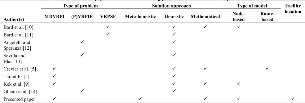
A summary of reviewed papers is presented in Table 1, according to which, LRPIRF has not received attention from researchers in terms of considering facility location phase.
Our aim in this paper is to initiate a node-based mixed integer linear programming model with a new kind of subtour elimination constraints to the LRPIRF, to consider facility location phase in this problem for the first time, and to solve the problem with genetic algorithm and tabu search approaches.
The paper is organized as follows: In section 2, we describe the problem. In section 3, we present the model formulation. In section 4, two solution approaches are discussed and finally in section 5, we discuss the results obtained when the algorithms are run on random instances and the sensitivity analysis is provided.
2. PROBLEM DESCRIPTION
Figure 1. An example of the LRPIRF with two intermediate replenishment facilities and six customers
TABLE 1. Review of some papers in the location routing problem with intermediate replenishment facilities
Author(s)
Type of problem Solution approach Type of model Facility
location MDVRPI (P)VRPIF VRPSF Meta-heuristic Heuristic Mathematical Node-based Route-based
Bard et al. [10] ü ü ü ü
Bard et al. [11] ü ü
Angelelli and Speranza [12]
ü ü
Sevilla and Blas [13]
ü ü
Crevier et al. [5] ü ü ü ü
Tarantilis [5] ü ü
Kek et al. [9] ü ü ü ü
Ghiani et al. [14] ü ü
Presented paper ü ü ü ü ü
The route of the vehicle in this instance is (0 1 2 A 3 4 5 B 6 0). So, three sub-routes are required to serve all six customers. The first sub-route starts from the depot at 0, continues to customers 1 and 2 and then the vehicle goes to intermediate facility A to replenish. After replenishment, second sub-route continues to customers 3, 4 and 5 and then the vehicle visits intermediate facility B. Similarly, the third sub-route continues to customer 6 and then the vehicle returns to the depot, completing its route.
3. MATHEMATICAL MODELING
The LRPIRF can be formulated as follows. Let
( )
VAG= , be a directed graph where
{
0, 1,..., ++1}
= v v vn r
V is the set of vertices in which the vertices v0 and vn+r+1 correspond to the start depot and the final depot, respectively (their locations are the same), Vc=
{
v1,...,vn}
is the customer set,{
n n n r}
r v v v
V = +1, +2,..., + is the set of r intermediate
replenishment facilities and A=
{
( )
vi,vj :vi,vjÎV,i¹j}
isthe arc set. Each arc (i,j)ÎV has a traveling cost per time unit, cij, and a traveling time, tij, which tight triangular inequality holds (i.e.,tij+tjk>tik). The origin
depot and all intermediate replenishment facilities have infinite supply. There is a single vehicle of capacity CAP located at the origin depot. A demand di is associated with each customer. At first decision, variables used in formulation are introduced:
ï î ï í ì =
0 1
ij
x
If the vehicle travels from node i to node j
Otherwise
,... 2 , 1 , 0
=
r
f The number of times intermediate facility is used for replenishment r
i
with these notations, we formulate the mathematical model: r r V r V i i jV j ij ij
ijt c CFf
x
Min
åå
å
Î Î ¹ Î + (1) 1 =
å
¹ Î i jV j ij x c V iÎ " (2)å
Î = c V j j vx0, 1 (3)
å
Î ++
=
c V
i n r
v i
x, 1 1 (4)
å
Î = c V j r rj f x r V rÎ " (5) 0 = -å
å
¹ Î ¹ Î j iV i ji j iV i ij x x V jÎ " (6) 0 } 1 , { } , 0 { = -å å
å å
+ +
Î Î
Î Î i Vrvn r jVc
ji r
V v
i jVc
ij x
x (7)
i
i d
u ³ "iÎVc (8)
CAP
ui£ "iÎVc (9)
ji i
i CAP d CAPx
u £ +( - )
} , { , 0 r c V v j V i Î " Î " (10) ji i j ij j i j x d d CAP CAPx CAP d u u ) ( - -+ + -+ ³ c c V j V i Î " Î " , (11) 0 , 1 = + + j
vn r
x "jÎV (12)
0
0 ,v = i
x "iÎVc (13)
0
=
i
u "iÎV\Vc (14)
{ }
0,1 Î ijx "i,jÎV,i¹j (15)
,... 2 , 1 , 0 = r
f "rÎVr (16)
0
³
i
u "iÎVc (17)
The objective (1) of this problem is to minimize the total service cost of customers including:
a) The cost of travelling:
åå
Î ¹ Î V i i jV j ij ij ijt c
x
b) The cost of using intermediate replenishment facilities: r r V r f CF
å
ÎEquation (2) ensures that each customer has exactly one successor that might be another customer, an intermediate facility, or the origin depot. Constraints (3) and (4) ensure that the vehicle passes through the depot exactly once. Constraints (5) ensure that the vehicle passes through any facility the number of times it is used for replenishment. Constraints (6) ensure conservation of flow at nodes. Constraints (7) ensure conservation of flow through the depot and facilities by
forcing the vehicle leaving the depot node to return to it. Constraints (8) to (11) are subtour elimination and capacity constraints [20]. The amount
u
i must be at least as large as the demand of customer i (8) and smaller than the capacity CAP of the vehicle (9). If customer i is the first of a tour,u
iis equal to thedemand of this customer. This is expressed through the three constraints (8), (9), and (10). Indeed, if i is the first customer of a tour,
x
ji is 1, so the constraint (10) is equivalent to the constraint (18).i
i d
u £ (18)
From (18), (8), and (9) we conclude that
u
i is equalto the demand of customer i. If i is not the first of a tour, then
x
ji is 0 and the constraint (10) is equivalent to the constraint (19), which is an extra constraint since constraints (8) and (9) include it.CAP
ui£ (19)
Suppose that i is not the first customer of the tour. Then,
u
i must equal the sum of demands served between either the depot or facilities and customer i, i.e. if customer j succeeds customer i in a tour, uj must beequal to the demand served on the tour from the depot to i, plus the amount ordered by j. This lies in the constraint (11). Indeed, if j comes immediately after i in a tour, xij is 1 and xji is 0, and the constraint (11) is equivalent to the constraint (20).
j i
j u d
u ³ + (20)
When j is not the immediate successor of i, constraint (11) remains valid. If j immediately precedes i, the constraint (11) becomes equal to (21).
i i
j u d
u ³ - (21)
This constraint means that the demand served from the depot to j is not smaller than the demand served between the depot and the successor i of j on the tour. Therefore, in addition to (21), the constraint (22) is obtained.
i j
i u d
u ³ + (22)
The combination of constraints (21) and (22) is equivalent to equation (23).
i j
i u d
u = + (23)
The constraint (24) is obtained when i and j are not next to each other. This constraint is redundant, since it is expressed by the constraints (8) and (9).
CAP d u
Constraints (12) and (13) complete the flow characterization by stemming the flow of the vehicle from the final depot and initiating it from the start depot, respectively. Constraints (14) initialize the load variables,
u
i to zero at the depot and all facilities.Constraints (15), (16) and (17) indicate that xij are
binary variables,
f
r are integer variables and the variablesu
i are non-negative.4. SOLUTION APPROACHES
4. 1. Genetic Algorithm It is quite time-consuming to solve the LRP on large scale due to our initial test using CPLEX. To solve the LRPIRF on a large scale, a Genetic Algorithm is proposed in this paper. GA is based on a parallel search mechanism that makes it more efficient than other optimization techniques [21]. It has been stated that the GA is capable to optimize globally in solving LRPs and VRPs [21-24].
Our GA approach begins by generating an initial chromosome set, each member of which corresponds to a feasible solution of the LRPIRF. A fitness function is used to rank chromosomes. In each generation, using an elite retaining approach, we choose fitter chromosomes from the population to be parents. This process iterates until a termination criterion is reached.
In summary, our methodology consists of seven components successively: (1) chromosome representation; (2) generation of the initial population; (3) fitness function; (4) selection process; (5) crossover operation; (6) mutation operation; and (7) termination criterion. The pseudocode for the genetic algorithm developed in this paper is presented in Table 2. The rest of this section describes these seven components.
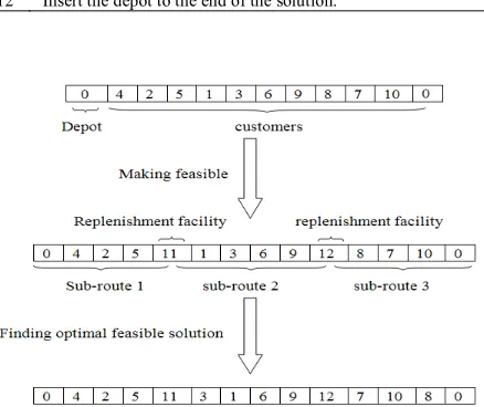
4. 1. 1 Chromosome Representation We use route representation to encode the chromosomes for the solution of the LRPIRF, in which the customers are listed in the order they are visited. In the example shown in Figure 2, there are 10 customers numbered from 1 to 10. The route representation for this instance is (0 4 2 5 1 3 6 9 8 7 10 0). Suppose that three routes are required to serve all customers. The first sub-route begins at the depot and continues to customers 4, 2 and 5, then the vehicle visits facility 11 to replenish. After replenishment, second sub-route continues to customers 1, 3, 6 and 9, then the vehicle visits replenishment facility 12 to replenish. Similarly, the third sub-route serves customers 8, 7 and 10, then the vehicle goes back to the depot. Solution infeasibility is coped with through a function, pseudocode of which is presented in Table 3.
TABLE 2. Pseudocode for the GA 1 Pi*← generate the initial population;
2 Evaluate the chromosomes in Pi;
3 while the termination criterion is not satisfied do 4 Po**← F
5 Repeat
6 Randomly select two parent chromosomes from Pi; produce two
offsprings from the parent chromosomes using crossover; and insert offsprings into Po;
7 until Po is full;
8 for each chromosome in Po do
9 Perform the mutation operation; 10 end for
11 Evaluate the chromosomes in Po;
12 P ← o
i P
P È ;
13 Pi← F
14 Insert the best chromosome of P into Pi;
15 By elitist strategy, select chromosomes from P to insert into Pi
until Pi is full;
16 end while
17 Return the best chromosome in Pi.
* Piis the initial population. ** Pois the offspring population.
TABLE 3. Pseudocode for the solution fix and feasibility 1 Exclude the depot and replenishment facilities from solution; 2 Insert the depot to the beginning of the solution;
3 While all customers are serviced;
4 Start summation of customers demands one by one from the beginning of the solution;
5 If the sum of demands exceeds the vehicle capacity; 6 Add a replenishment facility to the solution; 7 Set the summation of demands equal to 0; 8 go to 4;
9 else if
10 Continue the summation of demands; 11 end while
12 Insert the depot to the end of the solution.
4. 1. 2 Initial Population Initial population is created by random permutation of 1 to N, which N is the number of customers.
4. 1. 3 Fitness Function The GA ranks chromosomes based on the fitness function value. After the crossover and mutation operations, we attempt to improve the resultant offsprings in terms of the fitness function. At each generation, we use roulette wheel selection with fitness-based elite retaining approach with a fixed rate pe called recombination rate to make a
new population. With considering pcand pm as
crossover and mutation rates, respectively, pe is defined
as follows:
1 ( )
e c m
p = - p +p
Steps of this approach are presented below:
1. The fitness values of individuals are calculated. 2. According to the recombination rate, a set of
fittest individuals is selected for the reproduction.
3. Elite individuals are retained for the next generation.
Elitism method ensures that the best individual is transferred to the next generation and the best solution in each generation does not get worse.
4. 1. 4. Selection In each generation, the GA selects parents from the population set for the reproduction, and also selects members from the candidate set to form the population set for the next generation. We use the elitist roulette-wheel selection operator in this paper.
4. 1. 5. Crossover After selecting two parent chromosomes, the GA produces two offsprings using crossover operator. The crossover operator used here is one-point crossover where the cut point is selected randomly.
4. 1. 6. Mutation Mutation operations allow GA to explore wider in the solution space. In our GA, the insertion, swap, and inversion operators are used, which perform mutation on the set of offsprings produced by the crossover operations. The mutation probability of each offspring chromosome is equal to Pm. A substring is selected from the parent in a random manner and turns to form an offspring. The swap mutation works on one and the inversion mutation works on one or two chromosomes and both are used to increase the diversity of the population. In addition, the insertion mutation is not able to enhance routes.
4. 1. 7. Termination Criterion The GA continues until the number of iterations (generations) reaches a user-defined value.
4. 2. Tabu Search Algorithm In this section, a meta-heuristic solution approach for solving the LRPIRF model is presented. Tabu search is an iterative meta-heuristic for solving combinatorial problems. It has been stated that tabu search can find high quality solutions for the LRPs and VRPs compared to other meta-heuristics [25-29]. In this section, we describe the TS algorithm we implemented to solve the LRPIRF problem.
The basic concept of a TS algorithm is to repeatedly move from a current solution to another solution in a neighborhood of the current solution. Moving from current solution to another one is performed by small changes in current solution due to a set of rules in the neighborhood structure. The overall approach is to avoid cycling and getting trapped in local optimum by forbidding or penalizing moves which take the solution to the solution space previously visited i.e. tabu list. The difference between tabu search and other metaheuristic solution approaches is based on the concept of tabu list, a short term memory which is the storage place of some attributes of the previously visited solutions with prohibited moves. Therefore, it gives no permission to the revisited solutions and then avoids being trapped in the local optimum. If the forbidden move does not satisfy the aspiration criterion, only those moves that are not forbidden will be examined during the local search. The aspiration criterion used in this paper is better fitness, i.e. a move gets rid of the tabu list if it produces a solution with better fitness function value. TS method is terminated when the number of iterations reaches a user-defined value.
The pseudo-code for the Tabu Search algorithm developed in this paper is presented in Table 4.
5. DISCUSSION
The MIP model was programmed with CPLEX solver in GAMS 23.5.1 and the GA and TS codes were implemented in MATLAB R2012b, both run on AMD Phenom II Triple-Core Mobile Processor N830 (2.1GHz), 4GB RAM PC. In this research, computational results are obtained on a set of randomly generated instances and are compared in terms of solution time and objective function value. Tables 6 and 7 show the results.
TABLE 4. Pseudocode for the TS algorithm 1 Generate the initial solution s;
2 Develop the Tabu List;
3 While the set of the candidate solutions S is not complete; 4 Generate the candidate solution s from the current solution s; 5 Add s to S only if s is not forbidden or if the Aspiration
Criterion is satisfied;
6 Choose the best candidate solution s* in S ; 7 If fitness(s*) > fitness(s) then s = s*;
8 Update the Tabu List and the Aspiration Criteria; 9 If the termination condition met finish; 10 Otherwise go to Step 3.
TABLE 5. Tuned parameters of GA and TS
GA
Iteration=300
Population size=50
Crossover rate=0.7
Mutation rate=0.2
Recombination rate=0.1
TS Iteration=50 Tabu list=number of customers
Figure 3. Comparison of processing times
Figure 4. Comparison of objective function values
Table 6 shows that there is very small optimality gap between CPLEX and GA solutions such that in half of the instances the gap between solutions is zero. Even in instances 7-12, the available gap is not considerable. This is because the routing costs do not play an important role in increasing objective function value. In addition, the extreme convergence of GA solutions to lower bounds is because of using the same number of replenishment facilities. This implies that the proposed algorithm is so effective in satisfying the objective of the problem by minimizing the routing costs and using the optimal number of replenishment facilities i.e. minimizing facility location cost, which is obvious in all instances. The processing time of 5000 seconds in instances 11 and 12 means that their solution process has been stopped at that time. Therefore, the OFV obtained in that time is presented as the best known OFV.Due to Table 7 with the same instances as Table 6, there is not noticeable optimality gap between CPLEX and TS algorithm solutions. Like the GA, the convergence of TS algorithm solutions to lower bounds is because of minimizing routing costs and using the same number of replenishment facilities in all instances. This implies that the proposed Tabu Search algorithm is effective.
In instances 1, 3, 5, 7 and 9, the number of potential replenishment facilities is considered deliberately equal to the number of used replenishment facilities. But, in respectively equal-size instances 2, 4, 6, 8 and 10, the number of potential replenishment facilities is more than the number of used replenishment facilities, due to the location characteristic of the problem. As it is obvious, OFVs of equal-size instances in CPLEX are equal. This means that considering additional numder of replenishment facilities does not increase the OFV in CPLEX because CPLEX reaches lower bound in both instances. In spite of this, in instances with more-than-necessary number of facilities, complexity of the solution is high and the processing time is bigger than corresponding equal-size instances. In general, we conclude that considering more-than-necessary number of replenishment facilities increases problem complexity and solution time, but does not affect the OFV in CPLEX. This issue does not take place always in the GA and TS algorithm because they do not necessarily reach lower bound in all instances.
According to Figure 3, in terms of the processing time, the GA and TS algorithm work better than the optimality approach, in all instances. Even for large-scale instances 11 and 12, the processing times in GA and TS are lower than 50 seconds; but in order to obtain an upper bound of OFV for these intances, the solution process has been stopped at 5000 seconds in CPLEX. In addition, with increasing in customers number, the solution time in CPLEX increases exponentially. This implies that CPLEX in not practically able to solve the problem in large-scale instances.
0.1 1 10 100 1000 10000
1 2 3 4 5 6 7 8 9 10 11 12
pr
oc
essi
ng
ti
me
Instance number
CPLEX GA TS
400 450 500 550 600 650 700 750 800 850 900
1 2 3 4 5 6 7 8 9 10 11 12
O
FV
Instance number
TABLE 6. Comparison between CPLEX and Genetic Algorithm
Instance number
Number of customers
Number of potential replenishment facilities
CPLEX GA
OFV* Processing
time (s)
Number of used replenishmnet
facilities
OFV Processing
time (s)
Number of used replenishment
facilities
Optimality Gap (%)
1 5 1 441.184 3.391 1 441.184 0.236 1 0
2 5 4 441.184 3.469 1 441.184 0.426 1 0
3 6 1 442.974 3.696 1 442.974 0.453 1 0
4 6 4 442.974 3.811 1 442.974 0.856 1 0
5 8 2 655.807 16.155 2 655.807 2.170 2 0
6 8 4 655.807 19.691 2 655.807 2.188 2 0
7 9 2 666.471 108.737 2 669.884 10.89 2 0.51
8 9 4 666.471 151.148 2 682.440 11.52 2 2.33
9 10 2 736.993 619.322 2 742.224 12.26 2 0.7
10 10 4 736.993 718.563 2 748.770 13.714 2 1.57
11 11 4 801.385bk 5000 2 757.801 14.072 2 3.86
12 12 4 826.349bk 5000 2 773.894 14.553 2 5.02
OFV=Objective Function Value bk=best known
TABLE 7. Comparison between CPLEX and Tabu Search algorithm
Instance number
Number of customers
Number of potential replenishment facilities
CPLEX TS
OFV* Processing
time (s)
Number of used replenishment
facilities
OFV Processing
time (s)
Number of used replenishment
facilities
Optimality Gap (%)
1 5 1 441.184 3.391 1 441.184 0.548 1 0
2 5 4 441.184 3.469 1 441.184 0.824 1 0
3 6 1 442.974 3.696 1 442.974 0.938 1 0
4 6 4 442.974 3.811 1 442.974 1.149 1 0
5 8 2 655.807 16.155 2 655.807 5.231 2 0
6 8 4 655.807 19.691 2 680.158 5.867 2 3.58
7 9 2 666.471 108.737 2 708.593 10.384 2 5.94
8 9 4 666.471 151.148 2 723.890 11.492 2 7.93
9 10 2 736.993 619.322 2 764.472 16.430 2 3.59
10 10 4 736.993 718.563 2 773.573 18.293 2 4.73
11 11 4 801.385bk 5000 2 786.327 26.235 2 8.51
12 12 4 826.349bk 5000 2 798.528 33.552 2 8.41
OFV=Objective Function Value bk=best known
According to Figure 4, GA is better at converging to lower bounds in comparison with the TS algorithm in all instances. In addition, it is clear that there is a considerable increase in OFV from instance 4 to instance 5 in all solution approaches. This is because of the increase in problem size and specifically the need to use one more replenishment facility in instance 5. In large-size instances 11 and 12, CPLEX has been stopped at 5000 seconds and the best known OFV has been obtained as upper bound. Therefore, the corresponding OFVs in GA and TS are lower than this value.
6. CONCLUSION
in a reasonable time. Therefore, we propose a Genetic Algorithm and a Tabu Search algorithm to obtain near optimum solutions in large size instances and then compare them to determine the effectiveness of the algorithm. Computational results show that the proposed algorithms are efficient in terms of solution time and quality.
In terms of future research directions, the problem formulation can be extended to include the intermediate replenishment facilities with inventory costs and limited supply capacity. Considering multiple vehicles in the depot and facilities could also be examined.
7. REFERENCES
1. Sohrabi, B. and Bassiri, M., “Experiments to determine the simulated annealing parameters case study in VRP”,
International Journal of Engineering-Transactions B, Vol. 17, (2004), 71-80.
2. Nagy, G. and Salhi, S., “Location-routing: Issues, models and methods”, European Journal of Operational Research, Vol. 177, (2007), 649-672.
3. Wu, T. -H., Low, C. and Bai, J. -W., “Heuristic solutions to multi-depot location-routing problems”, Computers & Operations Research, Vol. 29, (2002), 1393-1415.
4. Setak, M., Karimi, H. and Rastani, S., “Designing incomplete hub location-routing network in urban transportation problem”,
International Journal of Engineering-Transactions C: Aspects, Vol. 26, (2013), 997-1006.
5. Tarantilis, C. D., Zachariadis, E. E. and Kiranoudis, C. T., “A hybrid guided local search for the vehicle-routing problem with intermediate replenishment facilities”, INFORMS Journal on Computing, Vol. 20, (2008), 154-168.
6. Crevier, B., Cordeau, J. -F. and Laporte, G., “The multi-depot vehicle routing problem with inter-depot routes”, European Journal of Operational Research, Vol. 176, (2007), 756-773. 7. Jordan, W. C. and Burns, L. D., “Truck backhauling on two
terminal networks”, Transportation Research Part B: Methodological, Vol. 18, (1984), 487-503.
8. Jordan, W. C., “Truck backhauling on networks with many terminals”, Transportation Research Part B: Methodological, Vol. 21, (1987), 183-193.
9. Kek, A. G., Cheu, R. L. and Meng, Q., “Distance-constrained capacitated vehicle routing problems with flexible assignment of start and end depots”, Mathematical and Computer Modelling, Vol. 47, (2008), 140-152.
10. Bard, J. F., Huang, L., Dror, M. and Jaillet. P., “A branch and cut algorithm for the VRP with satellite facilities”, IIE Transactions, Vol. 30, (1998), 821-834.
11. Bard, J.F., Huang, L., Jaillet, P. and Dror, M., “A decomposition approach to the inventory routing problem with satellite facilities”, Transportation Science, Vol. 32, (1998), 189-203. 12. Angelelli, E. and Speranza, G. M., “The periodic vehicle routing
problem with intermediate facilities”, European Journal of Operational Research, Vol. 137, (2002), 233-247.
13. Sevilla, F. C. and de Blas, C. S., “Vehicle routing problem with time windows and intermediate facilities”, SEIO Õ03 Edicions de la Universitat de Lleida, (2003), 3088-3096.
14. Ghiani, G., Laganà, D., Laporte, G. and Mari, F., “Ant colony optimization for the arc routing problem with intermediate facilities under capacity and length restrictions”, Journal of Heuristics, Vol. 16, (2010), 211-233.
15. Benjamin, A. and Beasley, J., “Metaheuristics for the waste collection vehicle routing problem with time windows, driver rest period and multiple disposal facilities”, Computers & Operations Research, Vol. 37, (2010), 2270-2280.
16. Jie, L., Dan, L., Min, L. and Yanfeng, H., “An improved multiple ant colony system for the collection vehicle routing problems with intermediate facilities”, 8th World Congress on Intelligent Control and Automation (WCICA), IEEE, (2010), 3078-3083.
17. Byung, K., Seongbae, K. and Surya, S., “Waste collection vehicle routing problem with time windows”, Computers & Operations Research, Vol. 33, (2006), 3624-3642.
18. AmiriFard, F. and Setak, M., “Comparison between Two Algorithms for Multi-Depot Vehicle Routing Problem with Inventory Transfer between Depots in a Three-Echelon Supply Chain”, International Journal of Computer Applications, Vol. 28, (2011), 39-45.
19. Hill, S.E., “Three Essays on the Location Routing Problem with Intermediate Storage Facilities”, Ph.D. Thesis, University of Alabama, (2008).
20. Guéret, C., Heipcke, S., Prins, C. and Sevaux, M., “Applications of optimization with Xpress-MP”, Dash Optimization Ltd., United Kingdom, (2005).
21. Derbel, H., Jarboui, B., Hanafi, S. and Chabchoub, H., “Genetic algorithm with iterated local search for solving a location-routing problem”, Expert Systems with Applications, Vol. 39, (2012), 2865-2871.
22. Marinakis, Y. and Marinaki, M., “A bilevel genetic algorithm for a real life location routing problem”, International Journal of Logistics: Research and Applications, Vol. 11, (2008), 49-65.
23. Cordeau, J. -F., Gendreau, M., Laporte, G., Potvin, J. -Y. and Semet, F., “A guide to vehicle routing heuristics”, Journal of the Operational Research Society, Vol. 53, (2002), 512-522. 24. Surekha, P. and Sumathi, S., “Solution To Multi-Depot Vehicle
Routing Problem Using Genetic Algorithms”, World Applied Programming, Vol. 1, (2011), 118-131.
25. Ghiani, G., Guerriero, F., Laporte, G. and Musmanno, R., “Tabu search heuristics for the arc routing problem with intermediate facilities under capacity and length restrictions”, Journal of Mathematical Modelling and Algorithms, Vol. 3, (2004), 209–
223.
26. Crainic, T., Sforza, A. and Sterle, C., “Tabu Search Heuristic for a Two-echelon Location-routing Problem”, CIRRELT, (2011). 27. Gupta, D. K., “Tabu Search for Vehicle Routing Problems
(VRPs)”, International Journal of Computer Mathematics,
Vol. 79, (2002), 693-701.
28. Khanh, P. N., Crainic, T. G. and Toulouse. M., “A Tabu Search for Time-dependent Multi-zone Multi-trip Vehicle Routing Problem with Time Windows”, European Journal of Operational Research, (2013).
A Node-based Mathematical Model towards the Location Routing Problem with
Intermediate Replenishment Facilities under Capacity Constraint
M. Setak, S. Jalili Bolhassani, H. Karimi
Faculty of Industrial Engineering, K. N. Toosi University of Technology, Tehran, Iran
P A P E R I N F O
Paper history:
Received 23 June 2013
Received in revised form 12 October 2013 Accepted 07 November 2013
Keywords:
Location Routing Problem
Intermediate Replenishment Facilities Mixed Integer Programming Capacity Constraint Genetic Algorithm Tabu Search
هﺪﯿﮑﭼ
نﺎﮑﻣﻪﻟﺎﺴﻣ،ﻪﻟﺎﻘﻣﻦﯾارد ﯽﺑﺎﯾ
-دﺪﺠﻣيﺮﯿﮔرﺎﺑﯽﻧﺎﯿﻣتﻼﯿﻬﺴﺗﺎﺑﯽﺑﺎﯾﺮﯿﺴﻣ
)
LRPIRF
(
ﯽﻣﯽﺳرﺮﺑار ﻪﻌﺳﻮﺗﻪﮐﻢﯿﻨﮐ
ﻪﺘﻓﺎﯾ نﺎﮑﻣﻪﻟﺎﺴﻣ ﯽﺑﺎﯾ
-ﯽﺑﺎﯾﺮﯿﺴﻣ
)
LRP
(
ﯽﻣﻪﯿﻠﻘﻧﻞﯾﺎﺳونآردﻪﮐﺖﺳا ﺪﻨﭼردﺪﻨﻧاﻮﺗ
ﻞﯿﻬﺴﺗ دﺪﺠﻣيﺮﯿﮔرﺎﺑ،ﯽﻧﺎﯿﻣ
ﺪﻨﻫدمﺎﺠﻧا
.
زاﻞﻣﺎﮐرﺎﺑﺎﺑﻪﯿﻠﻘﻧﻞﯾﺎﺳو ﻮﭘد
ﯽﻣﺖﮐﺮﺣﻪﺑعوﺮﺷ ﯽﻣﺲﯾوﺮﺳرﺎﺑمﺎﻤﺗاﺎﺗارنﺎﯾﺮﺘﺸﻣ،ﺪﻨﻨﮐ
ﯽﻣ،ﺪﻨﻫد ﺪﻨﻧاﻮﺗ
ﻪﺑدﺪﺠﻣيﺮﯿﮔرﺎﺑياﺮﺑ ﻞﯿﻬﺴﺗ
ﺖﻤﯾﺰﻋﯽﻧﺎﯿﻣ ﻪﺑنﺎﺷﺮﯿﺴﻣمﺎﻤﺗاﺖﻬﺟمﺎﺠﻧاﺮﺳو،ﺪﻨﻨﮐ
ﻮﭘد ﯽﻣزﺎﺑ ﺪﻧدﺮﮔ
.
،ﻪﻟﺎﻘﻣﻦﯾارد
ﺖﯾدوﺪﺤﻣزايﺪﯾﺪﺟعﻮﻧﺎﺑهﺮﮔﺮﺑﯽﻨﺘﺒﻣﻂﻠﺘﺨﻣﺢﯿﺤﺻدﺪﻋيﺰﯾرﻪﻣﺎﻧﺮﺑﯽﺿﺎﯾرلﺪﻣﮏﯾﻪﻟﺎﺴﻣﻦﯾاياﺮﺑ
فﺬﺣيﺎﻫ
رﻮﺗﺮﯾز ﯽﻣﯽﻓﺮﻌﻣ ﻢﯿﻨﮐ
.
نﺎﮑﻣزﺎﻓ،ﻪﯿﻠﻘﻧﻪﻠﯿﺳوﯽﺑﺎﯾﺮﯿﺴﻣزﺎﻓرﺎﻨﮐرد،ﻦﯾا ﺮﺑهوﻼﻋ ﯽﺑﺎﯾ
تﻼﯿﻬﺴﺗ ﻪﺘﻓﺮﮔﺮﻈﻧرد ﺰﯿﻧ
ﯽﻣ دﻮﺷ
.
ﻠﺌﺴﻣ فﺪﻫ ﺲﯾوﺮﺳ ﺖﻬﺟ ﻪﯿﻠﻘﻧ ﻞﯾﺎﺳو ياﺮﺑ ﺮﯿﺴﻣ ﻦﺘﻓﺎﯾﻪ ﻪﺑ نﺎﯾﺮﺘﺸﻣ ﻪﺑ ﯽﻫد
ﻪﻧﻮﮔ اﯾ
ﻪﮐ ﺖﺴ
ﺾﻘﻧ نوﺪﺑ
نﺎﮑﻣﻞﮐﻪﻨﯾﺰﻫوﺮﻔﺳ ﻞﮐﻪﻨﯾﺰﻫ،ﻪﯿﻠﻘﻧﻞﯾﺎﺳوﺖﯿﻓﺮﻇﺖﯾدوﺪﺤﻣ ﯽﺑﺎﯾ
تﻼﯿﻬﺴﺗ دﻮﺷﻪﻨﯿﻤﮐ
.
ﻪﻟﺎﺴﻣ
LRPIRF
ﻂﺳﻮﺗ
ﻞﺣ ﺮﮔ
CPLEX
مﺮﻧرد راﺰﻓا
GAMS 23.5.1
يﻮﺠﺘﺴﺟوﮏﯿﺘﻧژﻢﺘﯾرﻮﮕﻟايﺎﻫدﺮﮑﯾورو ﯽﻣﻞﺣعﻮﻨﻤﻣ
دﻮﺷ
.
ﺞﯾﺎﺘﻧ
ﯽﻣﺪﯿﻟﻮﺗﯽﻓدﺎﺼﺗترﻮﺻﻪﺑﻪﮐﻪﻧﻮﻤﻧﻪﻠﺌﺴﻣﻦﯾﺪﻨﭼﻖﯾﺮﻃزاﯽﺗﺎﺒﺳﺎﺤﻣ ﺑﺪﻧﻮﺷ
ﻪ ﯽﻣﺖﺳد ﻢﺘﯾرﻮﮕﻟاﯽﺋارﺎﮐوﺪﻨﯾآ يﺎﻫ
ﯽﻣنﺎﺸﻧباﻮﺟﺖﯿﻔﯿﮐوﻞﺣنﺎﻣزظﺎﺤﻟزا ارهﺪﺷدﺎﻬﻨﺸﯿﭘ ﺪﻨﻫد
.
doi:10.5829/idosi.ije.2014.27.06c.09