State Dependent Multi channel Queuing System with Ordered Entry

STATE DEPENDENT MULTI-CHANNEL QUEUING

SYSTEM WITH ORDERED ENTRY

M. Jain

Department of Mathematics, Institute of Basic Science Khandari, Agra 282002, India, [email protected]

C. Shekhar

D.A.V. (PG) College, Dehra Dun-248001 India, [email protected]

(Received: June 6, 2001 – Accepted in Revised Form: March 19, 2002)

Abstract In the present study, we analyze the multi-channel service system with ordered entry from finite-source and finite-storage at each channel. The arrival and service rates are assumed to be state dependent. The steady state probabilities of the system are obtained by using Chapmann-Kolmogorov equations. Some other performance indices viz. utilization of servers, expected number of units in the system and expected number of units at each channel have been derived. A computational algorithm is developed to determine the optimal allocation of storage space facilitated in front of three heterogeneous servers. Sensitivity analysis has been carried out to study the effect of variation of different parameters on the system performance.

Key Words Multi-Channel, Ordered Entry, State-Dependent, Chapmann-Kolmogorov Equations, Queue Size Distribution, Finite Source

ﻩﺪﻴﻜﭼ

ﻩﺪﻴﻜﭼ

ﻩﺪﻴﻜﭼ

ﻩﺪﻴﻜﭼ

ﺤﻣﻊﺒﻨﻣﺯﺍﻢﻈﻨﻣﻱﺩﻭﺭﻭﺎﺑﻪﻟﺎﻧﺎﻛﺪﻨﭼﺕﺎﻣﺪﺧﻢﺘﺴﻴﺳ،ﻪﻟﺎﻘﻣﻦﻳﺍﺭﺩ

ﻝﺎﻧﺎﻛﺮﻫﺭﺩﺩﻭﺪﺤﻣﻥﺰﺨﻣﻭﺩﻭﺪ

ﻲﻣﻲﺳﺭﺮﺑ ﺩﻮﺷ

.

ﻦﻤﭙﭼﺕﻻﺩﺎﻌﻣﻖﻳﺮﻃﺯﺍﻢﺘﺴﻴﺳﺕﺎﺒﺛ ﺖﻟﺎﺣﺕﻻﺎﻤﺘﺣﺍ

ﻲﻣﺖﺳﺪﺑﻑﻭﺮﮔﻮﻣﻮﻠﻛ ﺪﻳﺁ

. ﻱﺎﻬﺴﻳﺪﻧﺍ

ﻲﻨﻴﺑﺶﻴﭘﻱﺎﻫﺪﺣﺍﻭﺩﺍﺪﻌﺗﻭﻢﺘﺴﻴﺳﺭﺩﻩﺪﺷﻲﻨﻴﺑﺶﻴﭘﻱﺎﻫﺪﺣﺍﻭﺩﺍﺪﻌﺗ،ﻪﻣﺪﺧﻱﺭﺍﺩﺮﺑﻩﺮﻬﺑﺪﻨﻧﺎﻣﺮﮕﻳﺩﻲﺗﺎﻴﻠﻤﻋ

ﺖﺳﺍ ﻩﺪﺷﻪﺒﺳﺎﺤﻣﻝﺎﻧﺎﻛ ﺮﻫ ﺭﺩﻩﺪﺷ .

ﻟﺍ ﻚﻳ

ﻪﺳﻱﻮﻠﺟﺭﺩ ﻥﺰﺨﻣﻱﺎﻀﻓﻪﻨﻴﻬﺑ ﻲﺑﺎﻳﺎﺟ ﻱﺍﺮﺑ ﻲﺗﺎﺒﺳﺎﺤﻣﻢﺘﻳﺭﻮﮕ

ﺖﺳﺍ ﻩﺪﺷ ﻪﺘﺧﺎﺳ ﻥﮊﻭﺮﺘﻫ ﻡﺩﺎﺧ .

ﻢﺘﺴﻴﺳ ﺩﺮﻜﻠﻤﻋ ﺮﺑ ﻥﻮﮔﺎﻧﻮﮔ ﻱﺎﻫﺮﺘﻣﺍﺭﺎﭘ ﺮﻴﺛﺎﺗ ﻲﺳﺭﺮﺑ ﻱﺍﺮﺑ ﺖﻴﺳﺎﺴﺣ ﺰﻴﻟﺎﻧﺁ

ﺖﺳﺍﻩﺪﻳﺩﺮﮔﻡﺎﺠﻧﺍ .

1. INTRODUCTION

In many practical situations involving manufacturing, production, warehouses, computer and communication systems etc., the multi-channel queuing system with ordered entry and closed loop can be realized. The service may be transmission of a message, the repair of failed unit, the movement of a pallet, the movement of a

guided vehicle to assemble parts etc. In the manufacturing system, different channels serve the raw materials. The materials are transferred to different channels by closed loop conveyor. By facilitating the buffer facility at service channels, the number of lost or recirculation units can be reduced.

frame-works. Ordered unit multi-channel queuing system provides the service through many parallel servers where unit receives the service at first available channel. Disney [1,2] was the first researcher who discussed the two-channel closed loop conveyor model with ordered entry and homogeneous servers. Gupta [3] had extended the model given by Disney by considering the heterogeneous server and finite storage capacity. He considered two-channels which allowed a maximum threshold number of units for service and obtained steady state queue size distribution using generating function technique. Gumbel [4] studied a multi-chann el system with heterogeneous servers. Singh [5] investigated the queuing system for two and three channels with homogenous and heterogeneous servers . Pritsker [6] presented no-loss m-channel closed loop conveyor without storage at first (m- 1) channels and an infinite storage at the mth

channel so that the last channel processed all units taken from the conveyor. Gregory and Litton [7] studied m heterogeneous channel queuing system with ordered entry where the inter -arrival times are random multiples of a fixed time interval. They found that in order to minimize the number of lost units, the channel should be ordered by descending service rate. Lin and Elsayed [8] and Elsayed [9] studied heterogeneous multi-channel system with ordered entry and having the provision of storage capacity. Proctor, Elsayed and Elayat [10] investigated the three-channel conveyors system with ordered entry and without storage.

Balking is realistic phenomenon in many real life congestion situations wherein units may leave the queue in case of long queue or insufficient waiting space due to discouragement. In order to decrease the backlog and to check the balking behaviour of the jobs, the server may increase their service rate after a threshold level of unfinished jobs. These two considerations give the model a realistic touch that’s why we also consider the balking effect and faster service rate after a threshold level of unfinished jobs in our queuing system. Dick [11] derived some theorems on single server queue with balking. Jain [12] suggested diffusion approximation approach for G/G/1 double-ended queue with balking. A finite capacity priority queue with discouragement was studied by Jain and Singh [13]. Ke and Wang [14] evaluated

cost analysis of the M/M/R machine repair problem with balking, reneging and server breakdowns. Jain and Dhyani [15] proposed a state dependent bulk service queue with balking. Shawky [16] investigated the machine interference model with balking, reneging and spares.

We study the multi-channel queuing model with ordered entry and state dependent arrival and service rates in order to reduce the backlog, the service rate becomes faster as number of units exceed a pre-assigned the threshold value. The organization of the paper is as follows: The underlying notations and assumptions describing the model are outlined in Section 2. In Section 3, governing equations and their solution are presented. Various performance measures are presented in Section 4. The expression for cost function to allocate the storage space optimally is discussed in Section 5. The numerical algorithm to determine the optimal storage space subject to minimum cost is given in Section 6. In Section 7 sensitivity analyses to demonstrate the effect of different parameters on system performance measures, is performed by using numerical illustration. In the last section, the scope of the work and conclusion are drawn.

2. SYSTEM DESCRIPTION

The ordered entry queueing system with finite storage of different capacity at three channels is modeled. The following notations are used to describe the mathematical formulation of the model:

Z Finite source size

Kl The threshold value for l th

(l = 1, 2 & 3) channel after which channel provide the service with faster rate

λl Poisson arrival rate of customers at l th

(l = 1, 2 & 3) channel

µl Service rate for the l th

(l = 1, 2 & 3) channel

l

µ′ Faster service rate of respective channel when queue length reached to threshold level Kl

L,M,N Maximum storage space of 1st, 2nd and 3rd channels

P0, 0,0 Steady state probability that the system is

idle

Pi, j, k Steady state probability that there are i, j

and k units at first, second and third channels respectively

E (qi) Expected number of units in queue in front

of server i (i= 1, 2 & 3)

E (ni) Expected number of units at channel i (i=

1, 2 & 3) including the units in the service E (n) Expected number of units in the system

φ Utilization of the service channel

TC The total operating cost of the queueing system with three channels having storage capacities L, M and N.

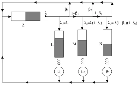
The system under consideration has the following characteristics:

• The customers arrive in Poisson fashion with parameter λ at channel 1. The customer may balk with probability β1 and β2 if the

storage space at first and second channels respectively are full so that the state dependent arrival rates λl(l=1, 2 & 3) at l

th

channels when there are i, j and k (0≤i≤L, 0≤j≤Μ & 0≤k≤Ν) customers at first, second and third channels, respectively, can be expressed as

λl(i, j, k) = (Z-i-j-k)λ

λ2(i, j, k) = (Z-i-j-k)λ(1−β1)

λ3(i, j, k) (Z-i-j-k)λ(1−β1)(1−β2)

• There is provision of storage space of size L, M and N in front of 1st, 2nd and 3rd channels respectively. An arrival occupies only one storage space.

• The units are served according to negative exponential distribution with parameters µ1,

µ2 and µ3 at respective channels.

• Kl(l=1, 2 & 3) is the threshold values of

respective channels at which the service rates of the servers increase in order to reduce backlog. Thus the state dependent service rates at respective channels are given by

  

≤ < µ′

≤ ≤ µ

= µ

L n K ;

K n 1 ; )

n (

1 1

1 1

1

  

≤ < µ′

≤ ≤ µ

= µ

M n K ;

K n 1 ; )

n (

2 2

2 2

2

and

  

≤ < µ′

≤ ≤ µ

= µ

N n K ;

K n 1 ; )

n (

3 3

3 3

3

• The queue discipline is ordered entry so that the arriving unit first checks the availability of storage space at first channel, if there is space for storage then it waits for its turn for service otherwise check the availability of storage space at the second and then at third channel. A graphical sketch of queueing system is shown in Figure 1.

3. MATHEMATICAL ANALYSIS

In this section, we formulate a Markovian model for the queuing system under study and outline the solution procedure by using matrix method. The steady state Chapmann-Kolmogorov equations governing the system are described as follows

0 P ) n ( P

) n ( P

) n ( P

Zλ_{1 0,0,0}+µ_{1 1,0,0}+µ_{2 0,1,0}+µ_{3 0,0,1}=

−

(1)

[

]

1 N ,..., 2 , 1 k ; 0 P

) n (

P ) n ( P

) n ( P

) n ( ) k Z (

1 k , 0 , 0 3

k , 1 , 0 2 k , 0 , 1 1 k , 0 , 0 3 1

− =

= µ

+

µ + µ

+ µ

+ λ − −

+

(2)

[

(Z−N)λ1+µ3(n)

]

P0,0,N+µ1(n)P1,0,N+µ2(n)P0,1,N=0

−

(3)

[

]

1 M ,..., 2 , 1 j 0

P ) n (

P ) n ( P

) n ( P

) n ( )

j Z (

1 , j , 0 3

0 , 1 j , 0 2 0 , j , 1 1 0 , j , 0 2 1

− =

= µ

+

µ + µ

+ µ

+ λ −

− ₊

[

]

1 N ,..., 2 , 1 k 1 M ,..., 2 , 1 j 0 P ) n ( P ) n ( P ) n ( P ) n ( ) n ( ) k j Z ( 1 k , j , 0 3 k , 1 j , 0 2 k , j , 1 1 k , j , 0 3 2 1 − = − = = µ + µ + µ + µ + µ + λ − − − + + (5)

[

]

1 M ,..., 2 , 1 j ; 0 P ) n ( P ) n ( P ) n ( ) n ( ) N j Z ( N , 1 j , 0 2 N , j , 1 1 N , j , 0 3 2 1 − = = µ + µ + µ + µ + λ − − − + (6)

[

]

0 P ) n ( P ) n ( P ) n ( ) M Z ( 1 , M , 0 3 0 , M , 1 1 0 , M , 0 2 1 = µ + µ + µ + λ − − (7)

[

]

1 N ,..., 2 , 1 k ; 0 P ) n ( P ) n ( P ) n ( ) n ( ) k M Z ( 1 k , M , 0 3 k , M , 1 1 k , M , 0 3 2 1 − = = µ + µ + µ + µ + λ − − − + (8)

[

]

0 P ) n ( P ) n ( ) n ( ) N M Z ( N , M , 1 1 N , M , 0 3 2 1 = µ + µ + µ + λ − − − (9)

[

]

1 L ,..., 2 , 1 i ; 0 P ) n ( P ) n ( P ) n ( P ) 1 i Z ( P ) n ( ) i Z ( 1 , 0 , i 3 0 , 1 , i 2 0 , 0 , 1 i 1 0 , 0 , 1 i 1 0 , 0 , i 1 1 − = = µ + µ + µ + λ + − + µ + λ − − + − (10)

[

]

1 N ,..., 2 , 1 k , 1 L ,..., 2 , 1 i ; 0 P ) n ( P ) n ( P ) n ( P ) 1 k i Z ( P ) n ( ) n ( ) k i Z ( 1 k , 0 , i 3 k , 1 , i 2 k , 0 , 1 i 1 k , 0 , 1 i 1 k , 0 , i 3 1 1 − = − = = µ + µ + µ + λ + − − + µ + µ + λ − − − + + − (11)

λ

β

1

1−β

1

β

2

1−β

2

λ

1

=λ

λ

2

=λ(1−β

1

) λ

3

= λ(1−β

1

)(1−β

2

)

µ

1

µ

2

µ

3

L

M

N

Z

[

]

1 L ,..., 2 , 1 i ; 0 P ) n ( P ) n ( P ) 1 N i Z ( P ) n ( ) n ( ) N i Z ( N , 1 , i 2 N , 0 , 1 i 1 N , 0 , 1 i 1 N , 0 , i 3 1 1 − = = µ + µ + λ + − − + µ + µ + λ − − − + − (12)

[

]

1 M ,..., 2 , 1 j 1 L ,..., 2 , 1 i 0 P ) n ( P ) n ( P ) 1 j i Z ( P ) n ( ) n ( ) j i Z ( 1 , j , i 3 0 , j , 1 i 1 0 , j , 1 i 1 0 , j , i 2 1 1 − = − = = µ + µ + λ + − − + µ + µ + λ − − − + − (13) 1 N ,..., 2 , 1 k 1 M ,..., 2 , 1 j 1 L ,..., 2 , 1 i 0 P ) n ( P ) n ( P ) n ( P ) 1 k j i Z ( P ) n ( ) k j i Z ( 1 k , j , i 3 k , 1 j , i 2 k , j , 1 i 1 k , j , 1 i 1 k , j , i 3 1 r r 1 − = − = − = = µ + µ + µ + λ + − − − +   

 _{− − − λ + µ}

− + + + − =

∑

(14) 1 M ,..., 2 , 1 j 1 L ,..., 2 , 1 i 0 P ) n ( P ) n ( P ) 1 N j i Z ( P ) n ( ) N j i Z ( N , 1 j , i 2 N , j , 1 i 1 N , j , 1 i 1 N , j , i 3 1 r r 1 − = − = = µ + µ + λ + − − − +   

 _{− − − λ + µ}

− + + − =

∑

(15)

[

]

1 L ,..., 2 , 1 i 0 P ) n ( P ) n ( P ) 1 M i Z ( P ) n ( ) n ( ) M i Z ( 1 , M , i 3 0 , M , 1 i 1 0 , M , 1 i 1 0 , M , i 2 1 1 − = = µ + µ + λ + − − + µ + µ + λ − − − + − (16) 1 N ,..., 2 , 1 k , 1 L ,..., 2 , 1 i ; 0 P ) n ( P ) n ( P ) 1 k M i Z ( P ) n ( ) k M i Z ( 1 k , M , i 3 k , M , 1 i 1 k , M , 1 i 1 k , M , i 3 1 r r 1 − = − = = µ + µ + λ + − − − +   

 _{− − − λ + µ}

− + + − =

∑

(17) 1 L ,..., 2 , 1 i 0 P ) n ( P ) 1 N M i Z ( P ) n ( ) N M i Z ( N , M , 1 i 1 N , M , 1 i 1 N , M , i 3 1 r r 1 − = = µ + λ + − − − +   

 _{− − − λ + µ}

− + − =

∑

(18)

[

]

0 P ) n ( P ) n ( P ) 1 L Z ( P ) n ( ) L Z ( 1 , 0 , L 3 0 , 1 , L 2 0 , 0 , 1 L 1 0 , 0 , L 1 2 = µ + µ + λ + − + µ + λ − − ₋ (19)

[

]

1 N ,..., 2 , 1 k ; 0 P ) n ( P ) n ( P ) 1 k L Z ( P ) n ( ) n ( ) k L Z ( 1 k , 0 , L 3 k , 1 , L 2 k , 0 , 1 L 1 k , 0 , L 3 1 2 − = = µ + µ + λ + − − + µ + µ + λ − − − + − (20)

[

]

0

P

)

n

(

P

)

1

N

L

Z

(

P

)

n

(

)

n

(

)

N

L

Z

(

N , 1 , L 2 N , 0 , 1 L 1 N , 0 , L 3 1 2

=

µ

+

λ

+

−

−

+

µ

+

µ

+

λ

−

−

−

− (21)

[

]

1 M ,..., 2 , 1 j ; 0 P ) n ( P ) n ( P ) 1 j L Z ( P ) 1 j L Z ( P ) n ( ) n ( ) j L Z ( 1 , j , L 3 1 , 1 j , L 2 0 , 1 j , L 2 0 , j , 1 L 1 0 , j , L 2 1 2 − = = µ + µ + λ + − − + λ + − − + µ + µ + λ − − − + − − (22) 1 N ,..., 2 , 1 k 1 M ,..., 2 , 1 j 0 P ) n ( P ) n ( P ) 1 k j L Z ( P ) 1 k j L Z ( P ) n ( ) k j L Z ( 1 k , j , L 3 k , 1 j , L 2 k , 1 j , L 2 k , j , 1 L 1 k , j , L 3 1 r r 2 − = − = = µ + µ + λ + − − − + λ + − − − +   

 _{− − − λ + µ}

1 M ,..., 2 , 1 j 0 P ) n ( P ) 1 N j L Z ( P ) 1 N j L Z ( P ) n ( ) N j L Z ( N , 1 j , L 2 N , 1 j , L 2 N , j , 1 L 1 N , j , L 3 1 r r 2 − = = µ + λ + − − − + λ + − − − +   

 _{− − − λ + µ}

− + − − =

∑

(24)

[

]

0 P ) n ( P ) 1 M L Z ( P ) 1 M L Z ( P ) n ( ) n ( ) M L Z ( 1 , M , L 3 0 , 1 M , L 2 0 , M , 1 L 1 0 , M , L 2 1 3 = µ + λ + − − + λ + − − + µ + µ + λ − − − − − (25) 1 N ,..., 2 , 1 k ; 0 P ) n ( P ) 1 k M L Z ( P ) 1 k M L Z ( P ) 1 k M L Z ( P ) n ( ) k M L Z ( 1 k , M , L 3 1 k , M , L 3 k , 1 M , L 2 k , M , 1 L 1 k , M , L 3 1 r r 3 − = = µ + λ + − − − + λ + − − − + λ + − − − +   

 _{− − − λ + µ}

− + − − − =

∑

(26)

[

]

0 P ) 1 N M L Z ( P ) 1 N M L Z ( P ) 1 N M L Z ( P ) n ( ) n ( ) n ( 1 N , M , L 3 N , 1 M , L 2 N , M , 1 L 1 N , M , L 3 2 1 = λ + − − − + λ + − − − + λ + − − − + µ + µ + µ − − − − (27)

The matrix method is used to solve the Equations 1-27, which can be written in matrix form as

AP = 0 (28)

where A is a square matrix of dimension (L+1)(M+1)(N+1) whose elements are the coefficients of state probabilities, P is the column matrix of steady state probabilities and 0 is null column matrix. All state probabilities of the system are calculated by imposing the normalizing condition 1 P L 0 i M 0 j N 0 k k , j , i =

∑∑∑

= = = (29)

so that Equation 28 can be written as

A1P + B = 0 (30)

where A1 is as same as A except that each element

of last raw is replaced by 1 and B is column vector whose last element is –1 and others are zero.

4. THE PERFORMANCE MEASURES

Now we establish some system performance for characterizing the model using steady state probabilities.

The expected number of units in queue for server r (r=1, 2 and 3) is given by

∑∑ ∑

= = = − = L 1 i M 0 j N 0 k k , j , i 1) (i 1)P

q ( E (31)

∑∑∑

= = = − = L 0 i M 1 j N 0 k k , j , i 2) (j 1)P

q ( E (32) and

∑∑∑

= = = − = L 0 i M 0 j N 1 k k , j , i 3) (k 1)P

q (

E (33)

The expected number of units in the system is obtained by

∑∑∑

= = = + + = L 0 i M 0 j N 0 k k , j , i P ) k j i ( ) n ( E (34)

  

 +

   

 

+ +

+

   

 

+ +

= φ

∑∑∑

∑∑

∑∑

∑∑

∑

∑

∑

= = =

= = = =

= =

= =

=

L

1 i

M

1 j

N

1 k

k , j , i

M

1 j

N

1 k

k , j , 0 L

1 i

N

1 k

k , 0 , i L

1 i

M

1 j

0 , j , i

N

1 k

K , 0 , 0 M

1 j

0 , j , 0 L

1 i

0 , 0 , i

P 3

P P

P 2

P P

P

(35)

5. OPTIMAL ALLOCATION

In order to set the optimal values of L, M and N, we construct a cost function using different cost elements as

   



 ₋

+

+ + + +

+ +

=

∑

∑

∑∑

∑∑

∑∑

=

= = = = =

= =

3

1 r

r r

6

3

1 r

r 5 4

L

0 i

M

0 j

0 , j , i 3 L

0 i

N

0 k

k , 0 , i 2

M

0 j

N

0 k

k , j , 0 1

) q ( E ) n ( E c

) q ( E c ) N M L ( c

P c

P c

P c

) N , M , L ( TC Minimize

(36)

subject to L+M+N = B (37) where

ci Cost per unit time when server i is idle

(i=1, 2 and 3)

c4 Cost of storage space per unit time

c5 Cost of waiting in storage space per

customer per unit time

c6 Cost per unit time a server spends serving

an arrival

Now the optimum allocation of storage spaces B among three channels so as to minimize the expected total cost given per unit time given in (37) can not be done using classical optimization technique such as branch and bound method as cost function is highly non-linear. For allocation purpose we shall use a direct search technique based on heuristic approach as discussed in the next section.

6. COMPUTATIONAL ALGORITHM

A computer program is developed in MATLAB to determine the steady-state probabilities using the direct method of conjugate gradient for solving the sparse system of equations. The flow chart for

Start

Stop λ , l, µÅ, Κ l, β l, β

B and Z

Read L= , M= , N=

Is L+M+N=B?

L++ or M ++ or N++

Construct A

Construct A &B Calculate P

Construct cost structure

Are all possible combination of L, M, N

taken such that L+M+N=B

Choose minimum total cost

Write L*, M*, N* Yes

No

No

Yes µ

l l

algorithmic procedure is shown in Figure 2. The algorithm used for numerical solution is summarized as follows:

Algorithm

Step1: Read the input parameters λl, µl, Kl,

l

µ′

(l=1, 2, 3), and βl, β2, B, Z.

Step 2: Take all possible combination of L, M, and N such that L+M+N = B

Step 3: Construct the transition matrix A.

Step 4: Construct the transition matrix A1 and

vector B.

Step 5: Solve the system of Equations 30 using the conjugate gradient method.

Step 6: Construct the cost structure and calculate the total expected cost using (36).

Step 7: Note L, M, and N (Say L*, M* and N*) at which total expected cost is minimum.

Step 8: Stop.

7. NUMERICAL RESULTS

For the validation of model developed in earlier section, extensive numerical experiment is performed. Computer program is developed in MATLAB to evaluate queue size distribution and other performance indices. The exhaustive enumeration procedure is used to determine the optimal value of L, M and N for the optimal allocation of finite storage space. The variation in performance measures of the system is depicted in Tables 1-3. In Table 1, the expected number of units in the system and the utilization of the service channels for λ = 0.5, β1 = 0.5 and β2 = 0.6 are

displayed with the variation of service rate for different population size. With the increase of service rate, the expected number of units and utilization of service channels decrease. The total operating cost with cost parameters c1= 20, c2 = 15,

c3 = 10, c4 = 5, c5 = 5, c6 = 50 is also tabulated. It is

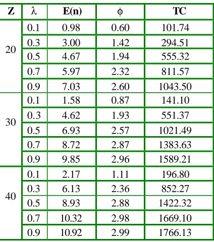
noted that it decreases gradually as µ increases. In Table 2, we demonstrate the same performance measures with the variation of arrival rate (λ) and population size (Z). It is easily observed that all performance indices increase with population size and arrival rate. Table 3 displays the performance measures with the variation of population size (Z) TABLE 1. Performance Measures by Varying Population

Size (Z) & Service Rate (µ).

Z µ E(n) φ TC

1.0 4.67 1.94 555.32 1.2 4.02 1.75 445.09 1.4 3.51 1.59 367.01 1.6 3.11 1.46 310.04 20

1.8 2.80 1.35 267.49 1.0 6.93 2.57 1021.49 1.2 6.04 2.34 831.11 1.4 5.35 2.14 688.90 1.6 4.78 1.98 581.38 30

1.8 4.31 1.84 498.36 1.0 8.93 2.88 1422.32 1.2 7.92 2.75 1226.40 1.4 7.05 2.59 1046.59 1.6 6.34 2.42 895.93 40

1.8 5.75 2.26 773.81

TABLE 2. Performance Measures by varying Population Size (Z) & Arrival Rate (λ).

Z λ E(n) φ TC

0.1 0.98 0.60 101.74 0.3 3.00 1.42 294.51 0.5 4.67 1.94 555.32 0.7 5.97 2.32 811.57 20

0.9 7.03 2.60 1043.50 0.1 1.58 0.87 141.10 0.3 4.62 1.93 551.37 0.5 6.93 2.57 1021.49 0.7 8.72 2.87 1383.63 30

0.9 9.85 2.96 1589.21 0.1 2.17 1.11 196.80 0.3 6.13 2.36 852.27 0.5 8.93 2.88 1422.32 0.7 10.32 2.98 1669.10 40

and balking rates (β1, β2). The decreasing trend is

observed in E(n), φ and TC with β1 and β2. In

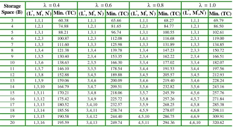
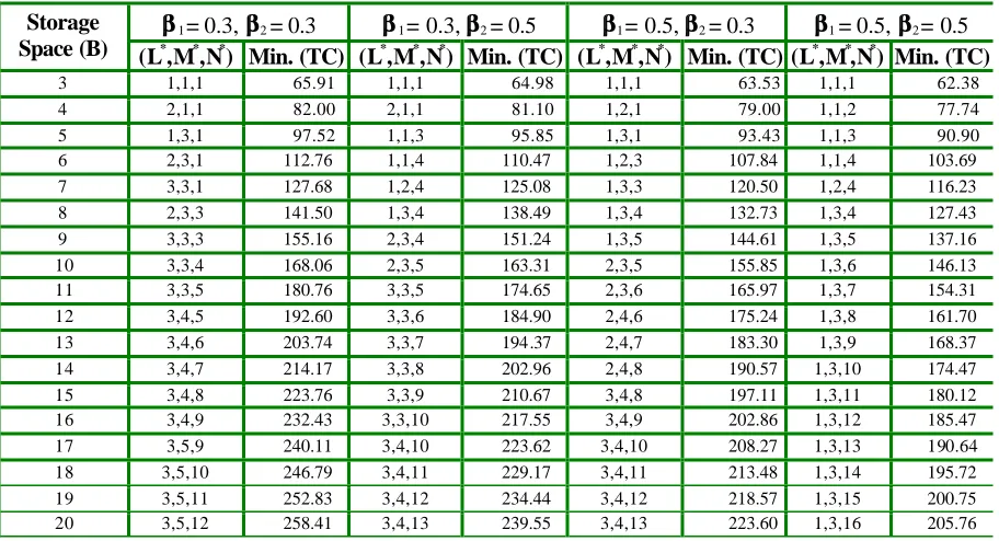
Tables 4 and 5, we show how the storage space is allocated optimally among three channels to

minimize the total operating cost of system with the variation of arrival and balking rates when (β1,β2) = (0.5,0.3) and λ = 0.5 respectively and

c1 = 12, c2 = 8, c3 = 4, c4 = 3, c5 = 15, c6 = 24, µ = 1.

TABLE 3. Performance Measures by Varying Population Size (Z) and Balking Rates (ββ11, , ββ22) .

E(n) φφ TC

Z β2

β1=0.2 β1=0.4 β1=0.6 β1=0.2 β1=0.4 β1=0.6 β1 = 0.2 β1=0.4 β1=0.6

0.0 6.41 5.48 4.41 2.51 2.26 1.90 962.50 759.50 523.79

0.2 6.20 5.34 4.36 2.46 2.21 1.87 914.46 723.17 508.00

0.4 5.95 5.19 4.31 2.39 2.15 1.84 852.91 681.01 491.16

0.6 5.67 5.04 4.26 2.27 2.06 1.81 774.73 632.68 473.35

20

0.8 5.38 4.89 4.21 2.11 1.96 1.77 678.43 578.50 454.72

0.0 9.81 8.97 7.28 2.95 2.89 2.65 1589.93 1440.53 1110.41

0.2 9.62 8.69 6.98 2.94 2.87 2.59 1557.03 1389.15 1046.56

0.4 9.29 8.26 6.62 2.9 2 2.82 2.51 1498.62 1305.82 963.16

0.6 8.65 7.59 6.21 2.86 2.71 2.37 1379.55 1164.82 857.64

30

0.8 7.43 6.69 5.81 2.65 2.45 2.18 1115.27 938.53 733.05

0.0 10.92 10.54 9.51 2.99 2.98 2.93 1771.24 1707.44 1529.38

0.2 10.84 10.39 9.23 2.99 2.98 2.91 1757.54 1683.91 1479.31

0.4 10.68 10.13 8.78 2.99 2.97 2.87 1732.27 1640.36 1394.58

0.6 10.33 9.58 8.03 2.98 2.94 2.76 1673.17 1542.09 1242.56

40

0.8 9.16 8.20 6.96 2.90 2.77 2.50 1462.13 1266.17 985.90

TABLE 4. Optimal Allocation (L*, M*, N*) of Storage Space by Varying Arrival Rate (λ).

λ = 0.4 λ = 0.6 λ = 0.8 λ = 1.0 Storage

Space (B) (L*

, M*, N*) Min. (TC) (L*, M*, N*) Min. (TC) (L*, M*, N*) Min. (TC) (L*, M*,N*) Min. (TC)

3 1,1,1 60.38 1,1,1 65.66 1,1,1 68.27 1,1,1 69.79

4 1,2,1 74.88 1,2,1 81.65 1,2,1 84.77 1,2,1 86.50

5 1,3,1 88.21 1,3,1 96.74 1,3,1 100.55 1,3,1 102.61

6 1,2,3 100.87 1,2,3 112.08 1,4,1 116.68 2,3,1 119.00

7 1,3,3 111.60 1,3,3 125.98 1,3,3 131.89 1,3,3 134.85

8 1,3,4 121.38 1,3,4 139.78 1,3,4 147.23 2,3,3 150.72

9 1,3,5 130.40 2,3,4 153.35 2,3,4 162.22 2,3,4 166.51

10 1,3,6 138.63 2,3,5 166.30 3,3,4 177.02 3,3,4 182.07

11 1,3,7 146.10 3,3,5 178.54 3,4,4 191.53 3,4,4 197.56

12 1,3,8 152.88 3,4,5 189.88 3,4,5 205.57 3,4,5 212.93

13 1,3,9 159.06 3,4,6 200.09 3,4,6 219.40 3,4,6 228.24

14 1,3,10 164.79 3,4,7 209.51 3,5,6 232.82 3,5,6 243.16

15 1,3,11 170.21 3,4,8 218.06 3,5,7 245.39 4,5,6 257.76

16 1,3,12 175.42 3,4,9 225.72 3,5,8 257.26 4,5,7 271.84

17 1,3,13 180.52 3,4,10 232.57 3,5,9 268.25 4,5,8 285.38

18 1,3,14 185.56 3,4,11 238.74 4,5,9 278.07 4,6,8 298.11

19 1,3,15 190.58 3,4,12 244.40 4,5,10 286.75 4,6,9 309.91

0 2 4 6 8 10 12

0.1 0.2 0.3 0.4 0.5 0.6 0.7 0.8 0.9

λλ E(n)

Z=20 Z=30 Z=40

2 4 6 8 10

1 1.2 1.4 1.6 1.8

µ µ E(n)

Z=20 Z=30 Z=40

(a) (b)

4 6 8 10 12

0 0.2 0.4 0.6 0.8

ββ1

E(n)

β=0.4 β=0.6 β=0.8

(c)

Figure 3. Expected number of units in the system E(n) by varying (a) arrival rate (λ), (b) service rate (µ) and (c) balking rates (β1, β2).

TABLE 5. Optimal Allocation (L*, M*, N*) of Storage Space by varying Balking Rates (ββ11ββ ,,22) .

ββ1 = 0.3,ββ2 = 0.3 ββ1 = 0.3,ββ2 = 0.5 ββ1 = 0.5,ββ2 = 0.3 ββ1 = 0.5,ββ2 = 0.5

Storage Space (B) _(L*

,M*,N*) Min. (TC) (L*,M*,N*) Min. (TC) (L*,M*,N*) Min. (TC) (L*,M*,N*) Min. (TC)

3 1,1,1 65.91 1,1,1 64.98 1,1,1 63.53 1,1,1 62.38

4 2,1,1 82.00 2,1,1 81.10 1,2,1 79.00 1,1,2 77.74

5 1,3,1 97.52 1,1,3 95.85 1,3,1 93.43 1,1,3 90.90

6 2,3,1 112.76 1,1,4 110.47 1,2,3 107.84 1,1,4 103.69

7 3,3,1 127.68 1,2,4 125.08 1,3,3 120.50 1,2,4 116.23

8 2,3,3 141.50 1,3,4 138.49 1,3,4 132.73 1,3,4 127.43

9 3,3,3 155.16 2,3,4 151.24 1,3,5 144.61 1,3,5 137.16

10 3,3,4 168.06 2,3,5 163.31 2,3,5 155.85 1,3,6 146.13

11 3,3,5 180.76 3,3,5 174.65 2,3,6 165.97 1,3,7 154.31

12 3,4,5 192.60 3,3,6 184.90 2,4,6 175.24 1,3,8 161.70

13 3,4,6 203.74 3,3,7 194.37 2,4,7 183.30 1,3,9 168.37

14 3,4,7 214.17 3,3,8 202.96 2,4,8 190.57 1,3,10 174.47

15 3,4,8 223.76 3,3,9 210.67 3,4,8 197.11 1,3,11 180.12

16 3,4,9 232.43 3,3,10 217.55 3,4,9 202.86 1,3,12 185.47

17 3,5,9 240.11 3,4,10 223.62 3,4,10 208.27 1,3,13 190.64

18 3,5,10 246.79 3,4,11 229.17 3,4,11 213.48 1,3,14 195.72

19 3,5,11 252.83 3,4,12 234.44 3,4,12 218.57 1,3,15 200.75

The corresponding minimum total cost is also illustrated.

The Figures 3(a)-(c) depict the expected number of units in the system E(n) by varying arrival rate (λ), service rate (µ) and balking rates (β1) for different value of population size (Z) and

balking rate (β2). With the increase in population

size, the expected number of units E(n) increases as shown in Figure 3(a) -3(b). In Figure 3(c), E(n) decreases with the increases in the value of β2.

Also E(n) increases with λ and decreases as µ and

β1 increases.

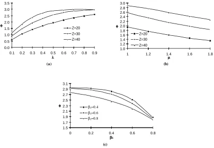
The graphs for the utilization of service channels (φ) vs. arrival rate (λ), service rate (µ) and β1 are

drawn in Figures 4(a)- 4(c) respectively by choosing the parameters as for Figures 3(a)-3(c). The effect of all parameters is noted and found the similar trends as for Figures 3(a)-3(c).

8. CONCLUSION

The ordered entry multi-channel queuing system with different storage capacities at heterogeneous three channels is studied. The cost model is developed to determine the optimal allocation of storage space among service channels. We have proposed an algorithm for optimal allocation of storage, based on heuristic approach, as the problem is too complicated to be solved by conventional optimization method. From the numerical experiment conducted in the present study, we have indicated the effect of operational parameters on the performance indices, thus enabling the system manager to make more robust decisions. Our study may be helpful in designing the manufacturing system where decisions have to be made with respect to the optimal space

0.0 0.5 1.0 1.5 2.0 2.5 3.0 3.5

0.1 0.2 0.3 0.4 0.5 0.6 0.7 0.8 0.9

λλ φφ

Z=20

Z=30

Z=40

1.0 1.2 1.4 1.6 1.8 2.0 2.2 2.4 2.6 2.8 3.0

1 1.2 1.4 1.6 1.8

µ µ φφ

Z=20

Z=30

Z=40

(a) (b)

1.5 1.7 1.9 2.1 2.3 2.5 2.7 2.9 3.1

0 0.2 0.4 0.6 0.8

ββ1

φφ _β2=0.4 β2=0.6 β2=0.8

(c)

allocation.

9. ACKNOWLEDGEMENT

University Grant Commission, New Delhi supports this work, vide project no. F. 8-5/98 (SI-R). The authors will like to acknowledge the helpful comments and suggestions of the anonymous referees.

10. REFERENCES

1. Disney, R. L., “Some Multi-Channel Queuing Problems with Ordered Entry”, J. Ind. Eng., Vol. 13, (1962), 46-48.

2. Disney, R. L., “Some Multi-Channel Queuing Problems with Ordered Entry - An Application to Conveyor Theory”, J. Ind. Eng., Vol. 14, (1963), 105-108.

3. Gupta, S. K. “Analysis of a Two Channel Queuing Problem with Ordered Entry”, J. Ind. Eng., Vol. 17, (1966), 54 -55.

4. Gumbel, H., “Waiting Lines with Heterogeneous Server”, Ops. Res., Vol. 8, (1960), 504-515.

5. Singh, V. P., “Markovian Queue with Three Heterogeneous Servers”, AIIE Trans., Vol. 3, (1971), 45-51.

6. Pritsker, A. A., “Application of Multi-Channel Queuing

Results to the Analysis of Conveyor Systems”, J. Ind. Eng., Vol. 17, (1966), 14-21.

7. Gregory, G. and Litton, C. D., “A Conveyor Model with Exponential Service Times”, Int. J. Prod. Res., Vol. 13, (1975), 1-7.

8. Elsayed, E. A., “Multi-Channel Queuing System with Ordered Entry and Finite Source”, Comput. Opn. Res.,

Vol. 10, No. 3, (1983), 213-222.

9. Lin, B. W. and Elsayed, E. A. “A General Solution for Multi-Channel Queuing Systems with Ordered Entry”,

Int. J. Comput. Ops. Res., Vol. 5, (1978), 219-225. 10. Proctor, C. L., Elsayed, E. A. and Elayat, H.,“A Conveyor

System with Homogeneous and Heterogeneous Servers with Dual Input”, Int. J. Prod. Res., Vol. 15, (1977), 73-85.

11. Dick, R. S., “Some Theorems on Single Server Queue with Balking”, Oper. Res., Vol. 18,(1970), 1193-1206. 12. Jain, M., “Diffusion Approximation for G/G/1 Double

Queue with Balking”, Int. J. Mgmt. Syst., Vol. 10, No. 2, (1994), 175 -180.

13. Jain, M. and Singh, C. J., “A Finite Capacity Priority Queue with Discouragement”, International Journal of Engineering, Vol. 11, No. 4, (1998), 191 -1 9 5 . 14. Ke, J. C. and Wang, K. H. “Cost Analysis of the M/M/R

Machine Repair Problem with Balking, Reneging and Server Breakdowns”, J. of Oper. Res. Soci., Vol. 50, (1999), 275-282.

15. Jain, M. and Dhyani, I., “A State Dependent Bulk Service Queue with Balking”, Opsearch, Vol. 36, No. 1, (1999), 70.

16. Shawky, A. I. “The Machine Interference Model: M/M/C/K/N with Balking, Reneging and Spares”,