Three-dimensional Vibration Suppression of an Euler-bernolli Beam via Boundary Control Method

Please cite this article as: A. Lotfavar, A. H. Mosalaeifard, Three-dimensional Vibration Suppression of an Euler-Brnoulli Beam via Boundary Control Method, International Journal of Engineering (IJE), TRANSACTIONS B: Applications Vol. 28, No. 5, (May 2015) 755-763

International Journal of Engineering

J o u r n a l H o m e p a g e : w w w . i j e . i r

Three-dimensional Vibration Suppression of an Euler-Bernoulli Beam via Boundary

Control Method

A. Lotfavar*a_{, A. H. Mosalaeifard}a,b

a _{Department of Mechanical and Aerospace Engineering, Shiraz University of Technology, Shiraz, Iran} b _{South Parss Gas Complex (SPGC), Asaloyeh, Iran}

P A P E R I N F O

Paper history:

Received 30 July 2014

Received in revised form 26 February 2015 Accepted 13 March 2015

Keywords:

Three-dimensional Vibrations Euler-Bernoulli Beam Boundary Control Method Fixed Beam

Rotary Beam

A B S T R A C T

In the present paper, general equations governing the beam vibration are derived in its three sub dimensions under the influence of system dynamics by using the Euler-Bernoulli beam theory and by utilizing Hamiltonian method. Then, two fundamental cases of a cantilever beam and a rotating beam are considered. Regarding the difficulty and the costliness of applying control commands to suppress the beam vibrations on its domain and regarding the difficulties of designing the controller based on the reduced and the discretized equations such as the control spillover and the boundary control method is both proposed and utilized. Thus, in order to suppress the beam vibration, control forces and moments placed on the system boundary are used. The controller which is designed based on the boundary control method and Lyapunov method guarantees the asymptotic stability of vibrations. The simulation results illustrate the high efficiency of the proposed method in suppressing the longitudinal and transversal vibrations of both states of cantilever and rotating beam with and without the boundary controller.

doi: 10.5829/idosi.ije.2015.28.05b.14

NOMENCLATURE

“×” Time derivative of the variable Vk

r

Velocity vector of typical point [m/s]

“׳” Derivative of a variable with respect to the spatial variable_{dummy variableh} x or _v Transverse deformation of beam in y direction in the Cartesian deformation coordinate system [m]

A Cross section area [m2_]

B Auxiliary function

W Work due to external forces and moments acting on the beam _[kg.m2_/s2 _{or J]}

E Modulus of elasticity [N/m2 _{or Pa]}

f Force [N]

w Transverse deformation of beam in z direction in the Cartesian _{deformation coordinate system [m]}

I Area moment of inertia [m4_]

k Positive constant

l Length [m]

x

r Longitudinal coordinate of typical point on the undeformed

beam [m]

M Moment [N.m]

m Mass [kg] Greek Symbols

rr Position vector of typical point on beam [m] δ Variational operator

0

rr Position vector of first end (base) of the beam [m] h Dummy variable [m]

T x y z w w w

é ù

W = ër û Angular velocity between two coordinate frames _[rad/s]

0 0 0 0

T

x y z

r _{= ë}éV V V ù_û

r& _{Rigid velocity of the moving frame [m/s]}

s Stretch variable [m] π Strain energy of the beam [kg.m2_/s2 _{or J]}

T Kinetic energy of the beam [kg.m2_/s2 _{or J] ρ Density [kg/m}3_]

t Time [s] _rr Deformation vector of typical point on beam respect to

undeformed beam [m]

u Longitudinal deformation of beam in the Cartesian deformation

coordinate system [m]

T u v w

rr& & & &= é_ë ù_{û Relative velocity of the typical point [m/s]}

*Corresponding Author’s Email: [email protected] (A. Lotfavar)

1. INTRODUCTION

Numerous mechanical systems can be considered as the combination of some rigid and some flexible parts. Rigid-Flexible complex dynamics of a flexible object can be modeled as the position and the orientation of the rigid part and vibrations of its elastic parts. It means that the dynamic effects of elastic parts on the whole system should be considered in the case that a desired performance is looked for. Interactions and the energy transfer between rigid and elastic motions of an object is highly important. A significant example was accrued in 1958 in the field of spacecraft dynamics, when the Explorer satellite was launched. The vibration of the antennae resulted in the energy transfer between rigid and elastic motions of the satellite and led to nutational instability [1]. Therefore, modeling the flexible parts and stabilizing their vibrations in order to control the resulting behavior have a major importance.

The beam, as a flexible object, is employed as the main element in many applications, since most of mechanical elements such as robot arms, rotating blades, and elastic space structures, especially flexible parts of spacecraft and satellites, are modeled as a beam [1]. Therefore, developing an accurate model for a beam vibration and designing a powerful controller for stabilizing its vibration are essential and have to be addressed.

Many researchers have studied the problems of modeling and controlling a beam vibration in many categories such as the flexible robot arms [2, 3], flexible structures and spacecrafts with flexible appendages [4, 5]. Most of researches on flexible beams are for one dimensional vibration of a cantilever beam attached to a fixed or a rotating base [6-11] while the vibrations in all three directions are coupled and influence each other, as well. Also, most of control approaches proposed for elastic systems, [1-11], rely mainly on discretizing the original partial differential equation (PDE) into a set of ordinary differential equations (ODE) by approximating and discretizing methods such as the finite element method (FEM), the finite assumed-modes method and other common methods [12].

But, it should be noted that an elastic system has an infinite modes that their degree of involvement in a system cannot be determined. Therefore, the approximate discretized model and its associated controllers can be high order and complex on condition that a large number of modes are considered. On the other hand, if some higher modes are neglected at the modeling step, the spillover instability and the ineffectiveness of the controller in high frequencies may occur under the discretized model based controller when the resulting controller is applied to the real system. Moreover, these methods need some devices and instruments such as strain gages or piezoelectric sensors and actuators [13-17] at some special interior points or

the distributed control action. Besides, in these methods location of sensors and actuators are important and several researches have been carried out to find their optimum locations [17, 18]. However, these methods are not applicable or they would be difficult, particularly for moving elastic objects [19].

Yoo et al. presented a large overall motion of a beam in 1995 [20]. They proposed a method based on the stretch deformation theory instead of the conventional axial deformation theory in order to have a more logical and accurate model especially for the high-speed rotary beam. In 2004, Liu and Hong studied three dimensional dynamics of a beam using of this theory [21].

Since last two decades, the boundary control (BC) method has been proposed by some researchers for PDE models of elastic systems [12, 19, 22-26]. The boundary control technique works based on the governing partial differential equations without any discretization or linearization. Besides, this technique needs some sensors and actuators which are placed on the boundary of systems. Under this condition, the boundary control procedure is an effective method to control elastic components.

In this paper, the boundary control method is proposed and is implemented for three-dimensional vibration suppression of an Euler-Bernoulli beam. In this case, the boundary control forces and torques are designed and the stability will be proved using a Lyapunov function and is verified by simulation results.

2. GOVERNING EQUATIONS

According to Figure 1, consider a homogenous and isotropic Euler-Bernoulli beam with lengthl, massm, densityr

( )

x , cross section areaA x

( )

, principal area moment of inertia I x_y

( )

andI x_z

( )

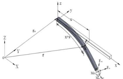
aboutyand z-axes, respectively. The beam which its elastic axis and the cross sections center line are coincident has a spatial rigid body motion.

Therefore, two coordinate systems are considered;

XYZ-frame as an inertial frame and xyz- frameas a moving frame which is attached to one end of the undeformed beam denoted by0. The beam is subjected to the boundary forces and moments F F Fsl, vl, wl,Mvl

and Mwl at the end which is denoted bylwhere F and

M stand for force and moment, and s v, andwfor longitudinal and the two lateral y and zdirections, respectively. Now, the three dimensional nonlinear partial differential equations of the Euler-Bernoulli beam vibrations are derived by the extended Hamiltonian method. Consequently, the kinetic and potential energies due to the rigid body motion and deformation should be considered as well as the external work which is performed by boundary forces and moments.

2. 1. The Kinetic Energy The deformation of a typical point kon the beam with respect to the undeformed beam is;

ˆ

ˆ ˆ

u i vj wk

rr= + + (1)

whereu x t( , ), v x t( , ) and w x t( , ) denote longitudinal and two transversal deformations of the beam in the Cartesian deformation coordinate system, respectively. To simplify the equation, the argument( , )x t is omitted.

The position vector of the typical point k with respect to the inertial frame can be presented as;

0

r rr r r= + +x rr (2)

whererr0 is the position vector of the first end of the beam and xr is the longitudinal coordinate of the typical point on the undeformed beam. Based on the transport theorem [1], the velocity of the typical point becomes;

(

)

(

)

(

)

(

)

(

)

0 0

0

0

ˆ

ˆ

ˆ

k x y z

y z x

z x y

V r V u w v i

V v x u w j

V w v x u k

= + + W ´ = + +

-+ + + +

-+ + + - +

r r_& r_& r r _&

& &

r r w w

w w

w w

(3)

where _{0 0 0 0} T

x y z

r _{= ë}éV V V ù_û

r& is the rigid velocity of the

moving frame, T

u v w

rr& & & &= é_ë ù_û the relative velocity of the

typical point, T

x y z

w w w

é ù

W = ër û the angular velocity

between two coordinate fames and “&” denotes time derivative of the variable. It is proper to mention that all of the vectors are presented based on the moving frame. Therefore, the kinetic energy of the beam becomes;

( )

₀

( ) ( )

1 1

2 2

l

k k k k

V

T=

òòò

V Vr r× r x dV=

ò

V Vr r× r x A x dx (4)

2. 2. The Potential Energy The strain energy can be written as;

( ) ( )

(

2

( )

2

( )

2

)

0

1 2

l

z y

E x A x s I x v I x w dx

p=

ò

¢ + ¢¢ + ¢¢ ₍₅₎

wheresis the stretch variable. According to the stretch deformation theory [20], it becomes;

(

2 2

)

0

1 2

x

s u= +

ò

v¢ +w d¢ h (6)

the prime denotes the derivative of a variable with respect to the spatial variablex or the dummy variable

h.

2. 3. The External Forces and Moments Work The work based on external forces and moments acting on the beam can be written as;

sl l vl l wl l vl l wl l

W f u= +f v+f w+ M v M w¢+ ¢ (7) where ul=u l t( , ), vl=v l t( , ) and w w l tl= ( , ).

2. 4. The Extended Hamilton’s Principle The extended Hamilton’s principle states that;

2

1

0 t

t T W dt

d

ò

é_ëp- - ù_û = (8)

where “d” denotes the variational operator, and t1 and 2

t are any two instances of time when t2> >t1 0. Substitution of Equations (4), (5) and (7) into Equation (8) and implementing some mathematical manipulations result in six equations for the rigid body motion of the beam as well as three equations for vibrations in three directions together with a set of terms for boundary conditions. Since in this research the problem of vibration control is studied, the coupled vibrational equations and the appropriate boundary conditions are considered as:

v The Equation of vibration in the non-Cartesian longitudinal direction s;

( ) ( )

( ) ( ) ( ) ( )

1 , 2 , z 3

( )

, y 0

E x A x s ¢ x A x B x té B x t B x t ù

é ù¢ + - + =

ë û r ë& w wû (9)

v The Equation of vibration in the transversal direction v;

( ) ( )

( )

( ) ( ) ( ) ( ) ( )

( ) ( ) ( ) ( ) ( )

1 2 3

1 2 3

, , ,

, , , 0

z sl

x

z y

l

z x

E x I x v f v

v A B t B t B t d

x A x B x t B x t B x t

¢¢

é ¢¢ù + ¢¢

ë û

¢

æ _{¢ é ù} ö

-ç_{è ë} - + _û ÷_ø

é ù

+ _ë + - _û=

ò

&

&

r h h h h w h w h

r w w

(10)

v The Equation of vibration in the transversal direction w;

( ) ( ) ( )

( ) ( ) ( ) ( ) ( )

( ) ( ) ( ) ( ) ( )

1 2 3

1 2 3

, , ,

, , , 0

y sl

x

z y

l

y x

E x I x w f w

w A B t B t B t d

x A x B x t B x t B x t

r h h h h w h w h

r w w

¢¢

é ¢¢ù + ¢¢

ë û

¢

æ _{¢ é ù} ö

-ç_{è ë} - + _û ÷_ø

é ù

+ _ë- + + _û=

ò

&

&

v A set of expressions for the boundary conditions;

( ) ( )

_{l sl} 0

E l A l s¢ +f = (E x I x v( ) ( )z ¢¢)¢_l+f vsl l¢-fvl=0

( ) ( )

(

E x I x wy ¢¢

)

¢_l+f wsl l¢-fwl=0E l I l v( ) ( )z l¢¢ +Mvl=0

( ) ( )

_{y l wl} 0

E l I l w¢¢+M =

(12)

where:

( )

1 , 0x y z

B x t =V + +u w& w -vw

( )

(

)

2 , 0y x z

B x t =V + -v w& w + +x uw

( )

(

)

3 , 0z x y

B x t =V + +w v& w - +x u w

( )

1 , 0x y y z z

B x t& =V& + +u w&& w& +w&w -vw& -v&w

( )

(

)

2 , 0y x x z z

B x t& =V& + -v w&& w& -w&w + +x uw& +u&w

( )

(

)

3 , 0z x x y y

B x t& =V& + +w v&& w& +v&w - +x uw& -u&w

(13)

Now, the equations can be simplified for two important cases; the fixed and the rotating cantilevers. Thus,

v The governing equations for the fixed based beam will be;

( ) ( )x A x u E x A x s( ) ( ) 0

r &&-é_ë ¢ù_û¢= (14)

( ) ( )x A x v v _lx ( ) ( )A ud E x I( ) ( )z x v ( )fslv 0

¢ _¢¢

æ _¢ ö _{é ¢¢ù ¢¢}

-ç_è ò ÷_ø+_{ë û} + =

&& &&

r r h h h (15)

( ) ( ) x ( ) ( ) ( ) ( )_y ( )_sl 0 l

x A x w&&-_èçæw¢ò A ud&& ö é_{÷ ëø}¢+ E x I x w¢¢ù_û¢¢+f w¢¢=

r r h h h (16)

v The governing equations for the rotary based beam around z-axis can be written as;

( ) ( )

₂

(

)

2

( ) ( )

₀

z z z

x A x u v v x u E x A x s

r _ëé&& &- w - w& - + wù_û- ¢¢= (17)

( ) ( )

(

( )

)

( ) ( ) ( ) 2 2 2 + 2 0 iv

z z z z sl

x

z z z

l

x A x v u v x u EI v f v

v A u v v u d

r w w w

r h h w w h w h

¢¢

+ - + + +

¢

æ _{¢ é ù} ö

-ç_è

ò

_ë - - - + _û ÷_ø =

& && &

&

&& & (18)

( ) ( )

( ) ( ) ₂ ( ) 2 ₀

iv

y sl

x

z z z

l

x A x w EI w f w

w A u v v u d

r

r h h w w h w h

¢¢

+ +

¢

æ _{¢ é ù} ö

-ç_è

ò

_ë - - - + _û ÷_ø =

&&

&

&& & (19)

3. THE CONTROLLER DESIGN

Regarding the main objective of the present paper, to suppress the coupled three dimensional vibrations of the assumed beam, the boundary control method is proposed without any discretization of the model and any avoidance of the control spillover. The recommended control scheme uses the system’s original governing PDE to produce control commands on the system boundaries. Stabilizing the system via using boundary

actions is so practical than utilizing control commands on the domain that are resulted by applying other methods such as piezo-actuators and piezo-sensors.

In order to stabilize the beam with the boundary control method a metric is defined as;

( ) ( )

( ) ( ) ( ) ( )

2 2 2 0

2 2 2

0 1 2 1 2 l l z y

V T U x A x u v w dx

E x A x s I x v I x w dx

r é ù

= + = _ë + + _û

é ¢ ¢¢ ¢¢ ù

+ _ë + + _û

ò ò

& & &

(20)

where the first term represents the kinetic energy, and the second one shows the potential energy due to the elongation and the two directional bending of the beam. This metric is a positive definite function of measure of closeness of the system states s v, _and w. That is chose based on idea of the Lyapunov function.

In order to apply the Lyapunov stability theorem to the parameter distributed system, the Zubov theorem [27] is employed. Now, it should be clarified that the time derivative of Equation (20) is negative definite. Therefore: ( ) ( ) ( ) ( ) ( ) ( ) 0 0 l l z y

V x A x uu vv ww dx

E x A x s s I x v v I x w w dx r

= éë + + ùû

é ¢ ¢ ¢¢ ¢¢ ¢¢ ¢¢ù

+ _ë + + _û

ò

ò

& _{&&& &&& && &}

& & & (21)

Substituting u v&& &&, and w&&from Equations (14)-(16) for Equation (21) gives;

( ) ( ) ( ) ( )

(

)

0 0 + l x z sl l x y sl l l z y

V EAs u v EAs d EI v f v v

w EAs d EI w f w w dx

E As s I v v I w w dx

h

h

é _¢ æ_{æ ¢ ö}¢ _¢¢ ö

ê ¢ ç ¢ ¢ ¢¢ ¢¢÷

= _ê - -_çç_è ÷_ø + + _÷

è ø

ë

ù

æ_{æ ¢ ö}¢ _¢¢ ö

ú

ç ¢ ¢ ¢¢ ¢¢÷

- -_çç_è ÷_ø + + _{÷ ú}

è ø û

é ¢ ¢+ ¢¢ ¢¢+ ¢¢ ¢¢ù

ë û

ò

ò

ò

ò

& _{& &}

&

& & &

(22)

However, Equation (6) can be written;

0 x

u s& &= -

ò

v v w w d¢ ¢& + ¢ ¢& h (23)

Replacing u& from Equation (23) with Equation (22) and collecting the terms give:

( ) ( )

(

)

( ) ( ) ( ) 0 0 0

0 0

0 0 l l z z l y y l l x x x l

V EAs s EAs s dx EI v v EI v v dx EI w w EI w w dx

EAs vv d dx EAs w w d dx

v v EAs d

h h

h

¢ ²

é _{¢ ¢ ¢}ù é _{¢¢ ¢¢ ¢¢} ù

= _ê + _ú + _ê - _ú

ë û ë û

²

é _{¢¢ ¢¢ ¢¢} ù

+ _ê - _ú

ë û

¢ ¢

é _{¢ ¢ ¢} ù é _{¢ ¢ ¢} ù

- _{ê ú} - _{ê ú}

ë û ë û

¢

é _{æ ö}ù

¢

ê _{ç ¢ ¢ ÷}

+ ê ç_è ÷_ø

êë

ò

ò

ò

ò

ò

ò

ò

ò

& _{& & & &}

& &

& &

& ( )

( ) ( )

0 0

0 0

l l x

l

l l

sl sl

dx w w EAs d dx

f v v dx f w w dx

h

¢

é _{æ ö}ù

¢

ú ₊ ê _{ç ¢ ¢ ÷}ú

ú ê ç_è ÷_øú

ú ê ú

û ë û

¢¢ ¢¢

-

-ò

ò

ò

ò

ò

&

& &

whereas it is possible to show;

(

)

₀

0 l

l

EAs s EAs s dx¢ EAs s

æ _{¢ + ¢ ¢}ö _{= é ¢ù}

ç ÷ ë û

è ø

ò

& & &

( ) ( )

0 ₀

l l

z z z z

EI v v EI v ²v dx EI v v EI v v¢

é _{¢¢ ¢¢- ¢¢} ù ₌é _{¢¢ ¢- ¢¢} ù

ê ú ê ú

ë û ë û

ò

& & & &

(

)

(

)

0

0 l l

y y y y

EI w w EI w ²w dx EI w w EI w w¢ é _{¢¢ ¢¢- ¢¢} ù ₌é _{¢¢ ¢- ¢¢} ù

ê ú ê ú

ë û ë û

ò

& & & &

0

0 ( 0 )

l l l

sl sl

f vv dx¢¢ =f vv¢ - v v dx¢ ¢

ò

& &

ò

&

0

0 ( 0 )

l l l

sl sl

f ww dx¢¢ =f ww¢ - w w dx¢ ¢

ò

& &

ò

&

(

)

(

)

(

)

0 0 0 0 l x

l l l

x

EAs vv d dx

EAs vv dx vv EAs d dx h h ¢ ¢ ¢ ¢ ¢ ¢ ¢ ¢ ¢¢ ¢ =

-ò

ò

ò

ò ò

& & & ( ) ( ) ( ) 0 0 0 x l l x l l l

v v EAs d dx

vv EAs d dx vv EAs dx

h

h

¢

æ _¢ ö

¢ ¢ ç ÷ ç ÷ è ø ¢ ¢ ¢¢ ¢ ¢ ¢ = + ò ò

ò ò ò

& & & ( ) ( ) ( ) 0 0 0 0 l x

l l l

x

EAs ww d dx

EAs ww dx ww EAs d dx h h ¢ ¢ ¢ ¢ ¢ ¢ ¢ ¢ ¢¢ ¢ =

-ò

ò

ò

ò

ò

& & & ( ) ( ) ( ) 0 0 0 x l l x l l l

w w EAs d dx

ww EAs d dx ww EAs dx

h

h

¢

æ _¢ ö

¢ ¢ ç ÷ ç ÷ è ø ¢ ¢ ¢¢ ¢ ¢ ¢ = + ò ò

ò ò ò

&

& &

(25)

Thus, Equation (24) becomes:

( )

(

)

0

0 0

0 0 0 0

( ) ( )

l l

l

z z y y

l l

l l

sl sl

V EAs s EI v v EI v v EI w w EI w w f vv v v dx f ww w w dx

¢

é ù

¢

é ù

¢ ¢¢ ¢ ¢¢ ¢¢ ¢ ¢¢

=é_ë ù_û +_ê - _ú +_ê - _ú

ë û ë û

¢ ¢ ¢ ¢ ¢ ¢

- -_ò - -_ò

& & & & & &

& & & &

(26)

Now, the terms can be replaced with the boundary equations Equation (12). Thus, collecting the terms gives: ( ) 0 ( ) l sl l

vl l wl l vl l wl l

sl l vl l wl l vl l wl l

V f s vv w w d

f v f w M v M w f u f v f w M v M w

h ¢ ¢ ¢ ¢ = - - + ¢ ¢ - - - -¢ ¢ = - - - -

-ò

& _{& & &} & & & &

& & & & &

(27)

Hence, to stabilize the beam vibrations, boundary forces and moments should be selected in a way that make V& negative. Consequently, it is possible to choose the boundary control actions as:

1

sl l

f =k u& (28)

2

vl l

f =k v& (29)

3

wl l

f =k w& (30)

4

vl l

M =k v&¢ (31)

5

wl l

M =k w&¢ (32)

where k k k k₁, , ,_{2 3 4} and k₅ are positive constants. Finally,

2 2 2 2 2

1l 2l 3 l 4l 5 l

V&= -k u& -k v& -k w& -k v&¢ -k w&¢ (33) This means that the time derivative of the metric equation meet zero when the system velocities become zero. According to Equations (28)-(32), when the system velocities converge to zero, the external forces and moments meet zero, too. Besides, corresponding to the governing equations when the terms related to the velocity and the external work are zero, the elastic potential terms converges to zero as well, and consequently the deflection becomes zero. Therefore, the beam vibrations get suppressed.

4. SIMULATION

In order to show the ability of the proposed control method, an aluminum beam with 1m length and a cross

section area _{2´0 .5cm}2 _{is considered. Density and}

modulus of elasticity of Aluminum are_{2710Kg m}3_and

70GPa, respectively. Simulation results are worked out for two cases of the fixed beam and the rotating beam with and without controller.

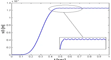
4. 1. The Fixed Beam In this case, it is assumed that the beam free end is subjected to 1mminitial displacement in the longitudinal direction and1cmin each transversal direction. Figures 2-4 illustrate the beam responses at the end and in the longitudinal and transversal directions due to initial displacements when there is no control action. As it is seen, vibrations keep on without any dissipation.

Now, the proposed controller is applied to the free end. In this case, the controller constants are considered as follows:

1 2 3 4 5 1

k =k =k =k =k = (34)

Figure 2. The stretch at the free end of the fixed beam without any controller

0 0.001 0.002 0.003 0.004 0.005 0.006 0.007 0.008 0.009 0.01 -1.5 -1 -0.5 0 0.5 1 1.5x 10

-3

t [sec]

s(

l)

Figure 3. The ytransversal vibration at the free end of the fixed beam without any controller

Figure 4. The ztransversal vibration at the free end of the fixed beam without any controller

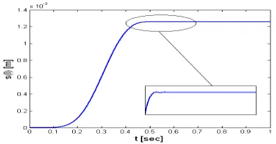
Figure 5. Eliminating the stretch at the free end of the fixed beam by the boundary controller

Figure 6. Eliminating the ytransversal vibration at the free end of the fixed beam by the boundary controller

Figures 5-7 demonstrate the beam end in the longitudinal and the transversal responses when the controller is present. In this case, the proposed controller has stabilized the beam vibration and provided a better performance for the beam.

Figure 7. Eliminating the ztransversal vibration at the free end of the fixed beam by the boundary controller

Figure 8. Controlled and uncontrolled tip transversal vibration using piezoelectric, [18]

Figure 9. The stretch at the free end of the rotating beam without any controller

Figure 10. Theytransversal vibration at the free end of the rotating beam and without controller

0 0.1 0.2 0.3 0.4 0.5 0.6 0.7 0.8 0.9 1 -0.015

-0.01 -0.005 0 0.005 0.01 0.015

t [s ec]

v(

l) [

m]

0 0.1 0.2 0.3 0.4 0.5 0.6 0.7 0.8 0.9 1 -0.015

-0.01 -0.005 0 0.005 0.01 0.015

t [sec]

w

(l)

[

m]

0 0.05 0.1 0.15 0.2 0.25 0.3 0.35 0.4 0.45 0.5

-1.5 -1 -0.5 0 0.5 1 1.5x 10

-3

t [sec]

s(

l) [

m]

0 0.1 0.2 0.3 0.4 0.5 0.6 0.7 0.8 0.9 1

-10 -8 -6 -4 -2 0 2 4 6 8x 10

-3

t [s ec ]

v(

l) [

m]

0 0.1 0.2 0.3 0.4 0.5 0.6 0.7 0.8 0.9 1 -12

-10 -8 -6 -4 -2 0 2 4x 10

-3

t [sec]

w

(l

) [

m]

0 0.1 0.2 0.3 0.4 0.5 0.6 0.7 0.8 0.9 1 -0.12

-0.1 -0.08 -0.06 -0.04 -0.02 0 0.02

t [sec]

v(

l)

Figure 11. Eliminating the stretch at the free end of the rotating beam by the boundary controller

Figure 12. Eliminating the ytransversal vibration at the free end of the rotating beam by the boundary controller

To show the power of the proposed boundary control method with respect to other conventional vibration control methods such as piezoelectric, the results can be compared to those of Kucuk et al. [18]. They have presented optimal vibration control of a vibrating Euler–Bernoulli beam based on the maximum principle and using piezoelectric patch actuators bonded to the top and bottom surfaces of the beam. As shown in Figure (8), they have succeeded to decrease amplitude of vibration linearly from 0.014 m to 0.002 m after 1 second but it has not been controlled completely. Whereas, based on Figure 2, the proposed boundary control method is able to vanish it asymptotically after 0.5 sec. It should be mentioned that the conventional methods such as using piezoelectric patches need to find the optimum location of sensors and actuators as well as they are based on discretized and reduced model of real beam while the proposed boundary control method does not do so.

4. 2. The Rotating Beam Since the proposed controller was able to suppress the fixed beam vibrations, it is suggested to be used for the rotating beam. In this case, it is assumed that the beam starts to accelerate from zero angular velocity to 3000rpm around the zaxis and keeps this speed. Figures 9-10 show the axial and transversal vibrations while the controller is not involved. In Figures 9 and 10, there are permanent vibrations due to the beam rotation. These vibrations should be suppressed. Thus, when the

boundary controller is included, the beam responses will be as shown in Figures 11 and 12. Moreover, it is observed that the proposed controller has rejected the undesirable vibrations. In comparing cantilever beam with the rotating one, it is understood that there is an initial peak which has resulted from the rotational speed of the system and its inertia. To decrease this peak, a passive control scheme should be considered in the designing time of the beam geometry and material. Concerning Figures 2-4 related to the cantilever beam and with regard to Figures 9-10 related to the rotating beam, constant amplitude vibrations are seen which are no structural damping in both cases of uncontrolled beam. However, concerning Figures 5-7 and 11-12, in the case of controlled beams the vibrations tend to vanish.

5. CONCLUSION

The governing equations of three dimensional vibrations of a moving Euler- Bernoulli beam are derived via the Hamiltonian method. These equations are simplified for two common cases; fixed and rotating cantilevers. The resulting equations are coupled with each other. The vibration in one direction as well as the rigid body motions of the beam causes three dimensional vibrations. Thus, the vibrations suppression is required. In conventional vibration control methods, the original partial differential equations are discretized to some algebraic or ordinary differential equations via some methods such as the finite elements method. However, these methods may lead the system to the state of controller spillover and instability. Hence, the boundary control method is implemented which is based on the original partial differential equations of the system and operates by some control forces and moments on the free end of the beam. It is apt to say that, the control actions are designed based on the energy of the system as the Lyapunov function and the metric. Consequently, the longitudinal and transversal vibrations for the fixed and the rotating cantilevers with and without any controller are simulated. The results illustrate that the beam vibrations are decreased quickly by this controlling method and there is no need to use distributed actuators on the domain to reject undesirable vibrations.

6. REFERENCE

1. Baruh, H., "Analytical dynamics, WCB/McGraw-Hill Boston, (1999).

0 0.1 0.2 0.3 0.4 0.5 0.6 0.7 0.8 0.9 1 -0.12

-0.1 -0.08 -0.06 -0.04 -0.02 0 0.02

t [sec]

v(

l)

2. Shin, H.-C. and Choi, S.-B., "Position control of a two-link flexible manipulator featuring piezoelectric actuators and sensors", Mechatronics, Vol. 11, No. 6, (2001), 707-729. 3. Karkoub, M. and Tamma, K., "Modeling and m-synthesis

control of flexible manipulators", Computers & Structures, Vol. 79, (2001), 543-551.

4. Hu, Q. and Ma, G., "Variable structure control and active vibration suppression of flexible spacecraft during attitude maneuver", Aerospace Science and Technology, Vol. 9, No. 4, (2005), 307-317.

5. Lacarbonara, W. and Yabuno, H., "Refined models of elastic beams undergoing large in-plane motions: Theory and experiment", International Journal of Solids and Structures, Vol. 43, No. 17, (2006), 5066-5084.

6. Yaman, M. and Sen, S., "Vibration control of a cantilever beam of varying orientation", International Journal of Solids and Structures, Vol. 44, No. 3, (2007), 1210-1220.

7. Khulief, Y., "Vibration suppression in using active modal control", Journal of Sound and Vibration, Vol. 242, No. 4, (2001), 681-699.

8. Cai, G.-P., Hong, J.-Z. and Yang, S.X., "Model study and active control of a rotating flexible cantilever beam", International Journal of Mechanical Sciences, Vol. 46, No. 6, (2004), 871-889.

9. Yang, J., Jiang, L. and Chen, D.C., "Dynamic modelling and control of a rotating euler–bernoulli beam", Journal of Sound and Vibration, Vol. 274, No. 3, (2004), 863-875.

10. Cai, G.-P., Hong, J.-Z. and Yang, S.X., "Dynamic analysis of a flexible hub-beam system with tip mass", Mechanics Research Communications, Vol. 32, No. 2, (2005), 173-190.

11. Canbolat, H., Dawson, D., Rahn, C. and Vedagarbha, P., "Boundary control of a cantilevered flexible beam with point-mass dynamics at the free end", Mechatronics, Vol. 8, No. 2, (1998), 163-186.

12. Cai, G.-P. and Lim, C., "Active control of a flexible hub-beam system using optimal tracking control method", International Journal of Mechanical Sciences, Vol. 48, No. 10, (2006), 1150-1162.

13. Chou, J.-H., Horng, R. and Liao, W.-H., "Robust observer-based OMF vibration control of flexible linkage mechanisms using piezoelectric films", International Journal of Mechanical Sciences, Vol. 40, No. 8, (1998), 749-759.

14. Moheimani, S., Pota, H. and Petersen, I., "Active control of vibrations in a piezoelectric laminate cantilevered beam", in Proceedings of International Symposium on Intelligent Robotic Systems, (1998), 505-512.

15. Indri, M. and Tornambe, A., "Robust trajectory tracking for flexible piezoelectric structures", IEE Proceedings-Control Theory and Applications, Vol. 141, No. 5, (1994), 289-294. 16. Alamatian, J. and Rezaeepazhand, J., "A simple approach for

determination of actuator and sensor locations in smart structures subjected to the dynamic loads", International Journal of Engineering-Transactions A: Basics, Vol. 24, No. 4, (2011), 341-349.

17. Sayyaadi, H. and Zakerzadeh, M., "Nonlinear analysis of a flexible beam actuated by a couple of active sma wire actuators",

International Journal of Engineering, Vol. 25, No. 3, (2012), 249-264.

18. Kucuk, I., Sadek, I.S., Zeini, E. and Adali, S., "Optimal vibration control of piezolaminated smart beams by the maximum principle", Computers & Structures, Vol. 89, No. 9, (2011), 744-749.

19. Lotfazar, A., Eghtesad, M. and Najafi, A., "Vibration control and trajectory tracking for general in-plane motion of an euler–

bernoulli beam via two-time scale and boundary control methods", Journal of Vibration and Acoustics, Vol. 130, No. 5, (2008), 51-62

20. Yoo, H., Ryan, R. and Scott, R., "Dynamics of flexible beams undergoing overall motions", Journal of Sound and Vibration, Vol. 181, No. 2, (1995), 261-278.

21. Liu, J. and Hong, J., "Dynamics of three-dimensional beams undergoing large overall motion", European Journal of Mechanics-A/Solids, Vol. 23, No. 6, (2004), 1051-1068. 22. Morgul, O., "Dynamic boundary control of a euler-bernoulli

beam", Automatic Control, IEEE Transactions on, Vol. 37, No. 5, (1992), 639-642.

23. Sallet, G., Xu, C. and Laousy, H., "Boundary feedback stabilization of a rotating body-beam system", in Decision and Control, Proceedings of the 34th IEEE Conference on, IEEE, Vol. 1, (1995), 930-935.

24. Fard, M. and Sagatun, S., "Exponential stabilization of a transversely vibrating beam via boundary control", Journal of Sound and Vibration, Vol. 240, No. 4, (2001), 613-622. 25. Chentouf, B., "Dynamic boundary controls of a rotating

body-beam system with time-varying angular velocity", Journal of Applied Mathematics, Vol. 2004, No. 2, (2004), 107-126. 26. Lotfavar, A. and Eghtesad, M., "Exponential stabilization of

transverse vibration and trajectory tracking for general in-plane motion of an euler–bernoulli beam via two-time scale and

boundary control methods", Journal of Vibration and

Acoustics, Vol. 131, No. 5, (2009), 54-63

Three-dimensional Vibration Suppression of an Euler-Bernoulli Beam via Boundary

Control Method

A. Lotfavara_{, A. H. Mosalaeifard} a,b

a_{Department of Mechanical and Aerospace Engineering, Shiraz University of Technology, Shiraz, Iran} b_{South Parss Gas Complex (SPGC), Asaloyeh, Iran}

P A P E R I N F O

Paper history:

Received 30 July 2014

Received in revised form 26 February 2015 Accepted 13 March 2015

Keywords:

Three-dimensional Vibrations Euler-Bernoulli Beam Boundary Control Method Fixed Beam

Rotary Beam

هﺪﯿﮑﭼ

ﺮﻠﯾواتﺎﯿﺿﺮﻓوﯽﻧﻮﺘﻠﯿﻤﻫشورزاهدﺎﻔﺘﺳاﺎﺑ،ﻪﻟﺎﻘﻣﻦﯾارد

-ﺮﯿﺛﺎﺗﺖﺤﺗﺪﻌﺑﻪﺳردﺮﯿﺗشﺎﻌﺗراﺮﺑﻢﮐﺎﺣﯽﻠﮐتﻻدﺎﻌﻣﯽﻟﻮﻧﺮﺑ

ﺖﺳاﻪﺘﻓﺮﮔراﺮﻗﺮﻈﻧﺪﻣراودﻪﯾﺎﭘوﺖﺑﺎﺛﻪﯾﺎﭘﺎﺑﺮﯿﺗﺖﻟﺎﺣودﺲﭙﺳوهﺪﺷجاﺮﺨﺘﺳانآﮏﯿﻣﺎﻨﯾد

.

يراﻮﺷدﻪﺑﻪﺟﻮﺗﺎﺑ ﻪﻨﯾﺰﻫو

ﺮﺑ

ﻢﮐﺎﺣتﻻدﺎﻌﻣسﺎﺳاﺮﺑﺮﻟﺮﺘﻨﮐﯽﺣاﺮﻃزاﯽﺷﺎﻧتﻼﮑﺸﻣوﺮﯿﺗﻪﻨﻣاديورردتﺎﺷﺎﻌﺗرافﺬﺣياﺮﺑﯽﻟﺮﺘﻨﮐرﻮﺘﺳدلﺎﻤﻋاندﻮﺑ ﺶﻫﺎﮐوﻪﺘﺴﺴﮔ ﺮﻟﺮﺘﻨﮐندﺮﮐﺰﯾرﺮﺳﺪﻨﻧﺎﻣﻪﺘﻓﺎﯾ

Control Spillover)

(

هﺪﺷهدﺎﻔﺘﺳاودﺎﻬﻨﺸﯿﭘيزﺮﻣلﺮﺘﻨﮐشورﻪﻟﺎﻘﻣﻦﯾارد

ﺖﺳا

.

ﻨﻣﻪﺑوﺎﺘﺳارﻦﯾارد وﺎﻫوﺮﯿﻧزا،ﺮﯿﺗتﺎﺷﺎﻌﺗرافﺬﺣرﻮﻈ

يﺎﻫروﺎﺘﺸﮔ ﺖﺳاهﺪﺷهدﺎﻔﺘﺳاﻢﺘﺴﯿﺳزﺮﻣردﻊﻗاوﯽﻟﺮﺘﻨﮐ

.

لﺮﺘﻨﮐ ﻪﯾﺎﭘﺮﺑهﺪﺷﯽﺣاﺮﻃﺮﮔ ﻪﺠﯿﺘﻧارتﺎﺷﺎﻌﺗراﯽﯾﺎﻤﻧيراﺪﯾﺎﭘﻒﻧﺎﭘﺎﯿﻟشورسﺎﺳاﺮﺑويزﺮﻣلﺮﺘﻨﮐي

ﺖﺳاهداد

.

ﻪﯿﺒﺸﺠﯾﺎﺘﻧ

-يزﺎﺳ ﺖﻟﺎﺣودﺮﻫياﺮﺑﯽﺿﺮﻋوﯽﻟﻮﻃتﺎﺷﺎﻌﺗرافﺬﺣياﺮﺑﺎﻫ لﺮﺘﻨﮐدﻮﺟونوﺪﺑﺞﯾﺎﺘﻧﻪﺴﯾﺎﻘﻣوراودوﺖﺑﺎﺛﺮﯿﺗ

ﺎﺑوﺮﮔ

لﺮﺘﻨﮐ ﺖﺳاﻪﺘﺷاديدﺎﻬﻨﺸﯿﭘشوريﻻﺎﺑﯽﯾﺎﻧاﻮﺗزانﺎﺸﻧيزﺮﻣﺮﮔ

.